Wave Walker DSP

DSP Algorithms for RF Systems

Buy the Book!

DSP for Beginners: Simple Explanations for Complex Numbers! The second edition includes a new chapter on complex sinusoids.

What is Power Spectral Density (PSD)?

February 1, 2024

Introduction

This blog describes the power spectral density (PSD) mathematically, algorithms for estimating the PSD, and real world challenges in PSD estimation. The analysis in this blog ignores the use of a windowing function for mathematical simplicity, but a windowing function should almost always be used in spectral analysis.

Check out these blogs:

Power Spectral Density (PSD) Mathematically

The instantaneous power of a signal x[n] is defined as

(1) $\begin{equation*}P_{x}[n] = |x[n]|^2 = x_{R}^2 + x_{I}^2\end{equation*}$

where

(2) $\begin{equation*}x_{R} = \text{RE}\left( x[n] \right),\end{equation*}$

(3) $\begin{equation*}x_{I} = \text{IM}\left( x[n] \right).\end{equation*}$

The DFT of x[n] is defined by

(4) $\begin{equation*}X[k] = \sum_{n=0}^{N-1} x[n]^{-j2\pi kn/N}\end{equation*}$

where N is the length of x[n] and the size of the DFT. The average power in the frequency domain, or power spectral density (PSD), is represented similarly to (1) [Lyons2011, p.63, p.140],

(5) $\begin{equation*}P_{X}[k] = |X[k]|^2 = X_{R}^2 + X_{I}^2.\end{equation*}$

The PSD represents the average power at each frequency bin k. Often the PSD is represented in dB,

(6) $\begin{equation*}\begin{split}P_{X,dB}[k] & = 10\text{log}_{10} \left( |X[k]|^2 \right) \\& = 20\text{log}_{10} \left( |X[k]| \right).\end{split}\end{equation*}$

When x[n] is known the PSD can be derived mathematically by finding X[k] followed by $P_{X}[k]$ , however it is a challenge when receiving unknown signals in a real world environment when a solution cannot be found analytically. In this case the PSD has to be estimated from the received signal.

Algorithms for PSD Estimation

A common problem in spectral analysis is being able to estimate the power spectral density $P_{X}[k]$ using a received signal. The two foundational tools for spectral estimation are:

Both the Bartlett and Daniell methods produce estimates of the PSD which may be referred to as periodograms [Oppenheim1999, p. 730]. Welch’s method is commonly used in spectral estimation but is a variation on the Bartlett method.

The objective is to produce the best PSD estimate with a finite data set. The following examples consider an input data length of 24 samples.

Bartlett's Method

Bartlett’s method computes several discrete Fourier transforms (DFT) over time with a smaller DFT size than the total data length and averages the results. For an example input sequence of 24 samples, consider the case in which an 8-point DFT is computed over each time segment and 3 DFTs are averaged together. The first DFT $X_{0}[k]$ would be computed over time segment $x[0], x[1], x[2], ~\dots, x[6], x[7]$ such that

(7) $\begin{equation*}X_{0}[k] = \mathcal{F} \{ x[0], x[1], x[2], ~\dots, x[6], x[7] \},\end{equation*}$

followed by the DFT over non-overlapping time series

(8) $\begin{equation*}X_{1}[k] = \mathcal{F} \{ x[8], x[9], x[10], ~\dots, x[14], x[15] \},\end{equation*}$

(9) $\begin{equation*}X_{2}[k] = \mathcal{F} \{ x[16], x[17], x[18], ~\dots, x[22], x[23] \}.\end{equation*}$

The power for each DFT would be computed according to (5),

(10) $\begin{equation*}P_{X_{0}}[k] = \left|X_{0}[k]\right|^2,\end{equation*}$

(11) $\begin{equation*}P_{X_{1}}[k] = \left|X_{1}[k] \right|^2,\end{equation*}$

(12) $\begin{equation*}P_{X_{2}}[k] = \left| X_{2}[k] \right|^2,\end{equation*}$

and averaged such that Bartlett’s PSD estimate is

(13) $\begin{equation*}\hat{S}_{X_{0,1,2}}[k] = \frac{1}{3} \left( P_{X_{0}}[k] + P_{X_{1}}[k] + P_{X_{2}}[k] \right).\end{equation*}$

Equation (13) can be generalized for M DFTs according to [Gardner1988, p.193],

(14) $\begin{equation*}\hat{S}_{X_{0,M-1}}}[k] = \frac{1}{M} \sum_{m=0}^{M-1} P_{X_{m}}[k] \\\end{equation*}$

or equivalently,

(15) $\begin{equation*}\hat{S}_{X_{0,M-1}}}[k] = \frac{1}{M} \sum_{m}^{M-1} |X_{m}[k]|^2.\end{equation*}$

Note that many textbook and online references average the magnitude squared as in (15). Averaging the power in dB is given by

(16) $\begin{equation*}\hat{S}_{X_{0,M-1},dB}}[k] = \frac{1}{M} \sum_{m=0}^{M-1} 20\text{log}_{10}\left( |X_{m}[k] \right).\end{equation*}$

Experimentally it would seem that averaging in dB (16) produces a smoother spectral response due to the compression in dB as the averages are not distorted by outliers as they would be in the linear domain. If you would be interested in this explanation please comment below and I will write a blog post about it.

Welch's Method

Welch’s method is a specific implementation of Bartlett’s method which uses 50% overlapping time series. Continuing with the example in (7) the DFTs are:

(17) $\begin{equation*}X_{0}[k] = \mathcal{F} \{ x[0], x[1], x[2], ~\dots, x[6], x[7] \},\end{equation*}$

(18) $\begin{equation*}X_{1}[k] = \mathcal{F} \{ x[4], x[5], x[6], ~\dots, x[10], x[11] \},\end{equation*}$

(19) $\begin{equation*}X_{2}[k] = \mathcal{F} \{ x[8], x[9], x[10], ~\dots, x[14], x[15] \},\end{equation*}$

(20) $\begin{equation*}X_{3}[k] = \mathcal{F} \{ x[12], x[13], x[14], ~\dots, x[18], x[19] \},\end{equation*}$

(21) $\begin{equation*}X_{4}[k] = \mathcal{F} \{ x[16], x[17], x[18], ~\dots, x[22], x[23] \}.\end{equation*}$

Due to the overlapping time-windows in (17) – (21) there are more DFTs to average which will require more computation but will also produce a smoother spectral response. Welch’s method is completed by averaging the power of the DFTs according to (16).

Welch’s method refers to exactly 50% overlap between successive time segments, however the amount of overlap can be varied based on the trade-offs between computation and desire for smoothness in the PSD estimate.

Daniell's Method

Where Bartlett’s method computes a smaller DFT and averages them over time, Daniell’s method takes a larger DFT and averages the frequency bins. For the same data length of N=24 samples, consider a 24-point DFT,

(22) $\begin{equation*}X[k] = \mathcal{F}\{ x[0], x[1], x[2], ~\dots, x[22], x[23] \}\end{equation*}$

whose power is

(23) $\begin{equation*}P_{X[k]} = |X[k]|^2.\end{equation*}$

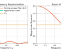
Daniell’s method averages the frequency bins in (23) using a convolution according to [Gardner1988, p.195]

(24) $\begin{equation*}\hat{S}_{X[k]} = P_{X[k]} * g[k]\end{equation*}$

where g[k] is a smoothing filter. The averaging can also be computed in dB according to

(25) $\begin{equation*}\hat{S}_{X[k],dB} = P_{X,dB}[k]} * g[k].\end{equation*}$

An example of g[k] is a moving average filter with length L,

(26) $\begin{equation*}g[k] =\begin{cases}1/L, & 0 \le k \le L-1, \\0, & \text{otherwise}.\end{cases}\end{equation*}$

PSD estimates (24) and (25) are computed through the convolution of an N-point DFT and smoothing filter g[k] with length L, producing an output of length N+L-1. The additional L-1 samples are invalid because they are outside the valid bounds of the PSD estimate only exist as a byproduct of the convolution. One method to handle the additional samples is to:

discard L-1 samples from the left side of the convolution (to remove all transients from the filtering)
extend the left most sample (L-1)/2 times
discard L-1 samples from the right side of the convolution
extend the right most sample (L-1)/2 times

If you have a better way to handle the transition areas with Daniell’s method please drop a comment below!

Conclusion

The Bartlett and Daniell methods are the two algorithms for estimating the power spectral density (PSD) of a given set of samples. Bartlett’s method computes a larger number of DFTs and averages them over time, whereas Daniell’s method computes a larger DFT but applies a smoothing filter over the frequency bins. Welch’s algorithm is a specific implementation of Bartlett’s method which includes the averaging of DFTs coming from 50% overlapping time segments. The analysis in this blog ignores the use of a windowing function for mathematical simplicity, but a windowing function should almost always be used in spectral analysis.