Wave Walker DSP

DSP Algorithms for RF Systems

Most Popular

Buy the Book!

DSP for Beginners: Simple Explanations for Complex Numbers! The second edition includes a new chapter on complex sinusoids.

Discrete Fourier Transform (DFT) of Complex Sinusoid
May 1, 2023

Table of Contents

Introduction

This blog derives the frequency response of a complex sinusoid using the discrete Fourier transform (DFT). The derivation starts by apply the discrete time Fourier transform (DTFT) of the complex sinusoid, simplifying the summation as a geometric series, and evaluating the DTFT at specific frequencies of the DFT.

Check out these other blogs:

Discrete Time Fourier Transform

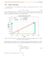
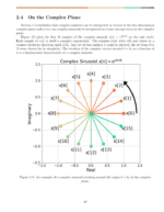
The discrete-time Fourier transform (DTFT) is defined as [Oppenheim1999, p.48]

(1)   \begin{equation*}X\left( e^{j\omega} \right) = \sum_{n=-\infty}^{\infty} x[n]e^{-j\omega n}. \end{equation*}

A realizable (ex: can be built in the real world) digital system must deal with signals which are finite length. A finite length complex sinusoid is defined according to

(2)   \begin{equation*}x[n] =\begin{cases}e^{j\omega_c n}, &  0 \le n \le N-1 \\0, & \text{otherwise}.\end{cases}\end{equation*}

Substituting (2) into (1),

(3)   \begin{equation*}\begin{split}X\left( e^{j\omega} \right) & = \sum_{n=0}^{N-1} e^{j\omega_c n}e^{-j \omega n} \\& = \sum_{n=0}^{N-1} e^{j \left( \omega_c - \omega \right) n }.\end{split}\end{equation*}

Geometric Series

The sum of m points in a finite length geometric series is defined as

(4)   \begin{equation*}S_{m} = \sum_{p=0}^{m-1} a r^{p}\end{equation*}

which is evaluated as (reference)

(5)   \begin{equation*}S_{m} = \frac{a\left( 1-r^m \right)}{1-r}.\end{equation*}

The result in (3) can be written as the geometric series with terms

(6)   \begin{equation*}a = 1,\end{equation*}

(7)   \begin{equation*}r = e^{j\left( \omega_c - \omega \right),\end{equation*}

(8)   \begin{equation*}m = N.\end{equation*}

Substituting (6)-(8) into (5),

(9)   \begin{equation*}X\left( e^{j\omega} \right) = S_{N} = \frac{1-e^{j\left(\omega_c - \omega\right)N}}{1-e^{j\left(\omega_c - \omega\right)}}.\end{equation*}

Applying L'Hospital's Rule

Equation (9) is undefined when \omega = \omega_c therefore L’Hospital’s rule is applied,

(10)   \begin{equation*}X\left( e^{j \omega} \right) |_{\omega=\omega_c} = \dfrac{\frac{\partial}{\partial \omega} \left(  1-e^{j\left(\omega_c - \omega\right)N  \right)}}{\frac{\partial}{\partial \omega} \left(  1-e^{j\left(\omega_c - \omega\right)  \right)}}.\end{equation*}

Simplifying (10),

(11)   \begin{equation*}\begin{split}X\left( e^{j \omega} \right) |_{\omega=\omega_c} & = \frac{-jNe^{j\left( \omega_c - \omega\right)N}}{-je^{j\left( \omega_c - \omega\right)}} \\& = Ne^{j\left( \omega_c - \omega \right) \left(N-1\right)} \\& = N.\end{split}\end{equation*}

The frequency response can therefore be written as

(12)   \begin{equation*}X\left( e^{j \omega}\right) = \begin{cases}\dfrac{1-e^{j\left(\omega_c - \omega\right)N}}{1-e^{j\left(\omega_c - \omega\right)}}, & \omega \neq \omega_c \\N, & \omega = \omega_c.\end{cases}\end{equation*}

Discrete Fourier Transform (DFT) of Complex Sinusoid

The DFT is a simplified case of the DTFT where the frequencies \omega are only evaluated at

(13)   \begin{equation*}\omega = \frac{2\pi k}{N}\end{equation*}

where k = 0, 1, 2, \dots, N-1, [Oppenheim1999, p.542]. Substituting (13) into (12),

(14)   \begin{equation*}X[k] = \begin{cases}\dfrac{1-e^{j\left(\omega_c - 2\pi k/N\right)N}}{1-e^{j\left(\omega_c-2\pi k/N\right)}}, & 2\pi k/N \neq \omega_c \\N, & 2\pi k/N = \omega_c.\end{cases}\end{equation*}

The DFT (14) can be further simplified as 

(15)   \begin{equation*}X[k] = \begin{cases}e^{j\alpha\left(N-1\right)/2}\cdot \dfrac{\sin\left( \alpha N/2 \right)}{\sin \left( \alpha/2 \right)}, & 2\pi k/N \neq \omega_c, \\N, & 2\pi k/N = \omega_c.\end{cases}\end{equation*}


Comparing to Simulation

Figures 1-3 compare equation (15) to NumPy’s DFT function for sinusoids with frequencies \omega_c = \pi/4, 3\pi/4, 0.57\pi and N=4096.

Figure 1: The discrete Fourier transform (DFT) of a complex sinusoid with frequency pi/4.
Figure 2: The discrete Fourier transform (DFT) of a complex sinusoid with frequency 3pi/4.
Figure 3: The discrete Fourier transform (DFT) of a complex sinusoid with frequency 0.57pi.

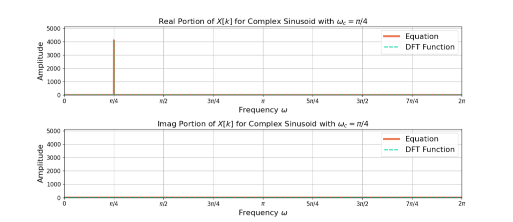
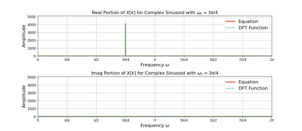
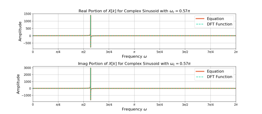
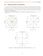
You may have noticed that all of the sinusoid’s energy is contained within a single bin when \omega_c is of the form 2 \pi k / N as in Figures 1 and 2. For Figure 3, the energy is spread across multiple frequency bins. Figure 4 shows a zoomed in version of Figure 3 for more clarity.

Figure 4: The discrete Fourier transform (DFT) of a complex sinusoid with frequency 0.57pi (zoom view).

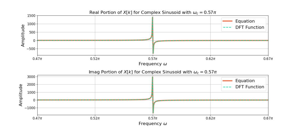
The sinusoid’s energy is spread across multiple bins because the sinusoid does not complete an integer number of cycles of frequency \omega_c in N samples. This effect is related to the frequency resolution of the DFT.

Conclusion

The discrete time Fourier transform (DTFT) and discrete Fourier transform (DFT) of a complex sinusoid were derived. The analytic equation was compared for correctness against a numerical DFT function. 

Check out these other blogs:

Leave a Reply

God, the Lord, is my strength; he makes my feet like the deer’s; he makes me tread on my high places. Habakkuk 3:19

This website participates in the Amazon Associates program. As an Amazon Associate I earn from qualifying purchases.

© 2021-2023 Wave Walker DSP