
![A BPSK signal s[n], real Gaussian noise w[n], and the received signal x[n] = s[n] + w[n] for SNR = 20 dB](https://www.wavewalkerdsp.com/wp-content/uploads/wordpress-popular-posts/15621-featured-125x100.png)

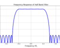
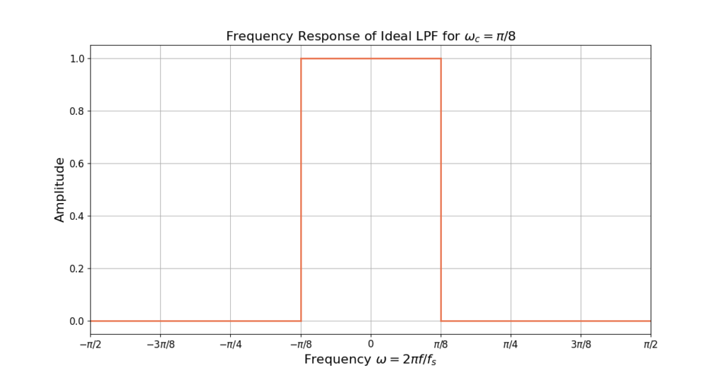
An ideal low pass filter (LPF) allows signals below the cutoff frequency  to pass through unmodified with a linear gain of 1 and no phase change, while simultaneously completely rejecting all frequencies above the cutoff frequency with a linear gain of 0.
Mathematically, the ideal LPF is defined in the frequency domain by [oppenheim1999, p.43]
(1) 
The frequency response for the ideal LPF in (1) for  is given in Figure 1.
The ideal LPF in the time domain is derived by taking the inverse discrete-time Fourier transform (IDTFT) of (1),
(2) ![\begin{equation*}h[n] = \mathcal{F}^{-1} \left\{ H\left( e^{j\omega} \right) \right\}.\end{equation*}](https://www.wavewalkerdsp.com/wp-content/ql-cache/quicklatex.com-2c076b16eb939298d22c39df8cd558c9_l3.png "Rendered by QuickLaTeX.com")
The IDTFT is defined as
(3) ![\begin{equation*}x[n] = \frac{1}{2\pi} \int_{-\pi}^{\pi} X\left( e^{j\omega} \right) e^{j\omega n}d\omega.\end{equation*}](https://www.wavewalkerdsp.com/wp-content/ql-cache/quicklatex.com-8dafb7a6e93c5b4cf10be9339c4f08d1_l3.png "Rendered by QuickLaTeX.com")
(4) ![\begin{equation*}h[n] = \frac{1}{2\pi} \int_{-\omega_c}^{\omega_c} e^{j\omega n} d\omega.\end{equation*}](https://www.wavewalkerdsp.com/wp-content/ql-cache/quicklatex.com-28659a66d16e12635c5590478810e4b1_l3.png "Rendered by QuickLaTeX.com")
The integral in (4) is simplified via Euler’s formula as
(5) ![\begin{equation*}\begin{split}h[n] & = \frac{1}{j2\pi n} e^{j \omega n} \Big|_{-\omega_c}^{\omega_c} \\& = \frac{1}{j2\pi n} \left( e^{j\omega_c n} - e^{-j\omega_c n} \right) \\& = \frac{1}{\pi n} \sin \left( \omega_c n \right). \\\end{split}\end{equation*}](https://www.wavewalkerdsp.com/wp-content/ql-cache/quicklatex.com-41452002ff4da11d2c1cd60a5f820ad7_l3.png "Rendered by QuickLaTeX.com")
The cutoff frequency is the frequency in radians, defined as
(6) 
where  is the frequency
  in Hz normalized by the sampling rate
  ,
,
(7) 
The impulse response h[n] can therefore be written as
(8) ![\begin{equation*}h[n] = \frac{1}{\pi n} \sin \left( 2\pi f_{n} n \right).\end{equation*}](https://www.wavewalkerdsp.com/wp-content/ql-cache/quicklatex.com-1846e7e60d74b08bfa9debf87f3498fa_l3.png "Rendered by QuickLaTeX.com")
Equation (8) can then be transformed into a sinc function where
(9) 
The impulse response h[n] can therefore be written as
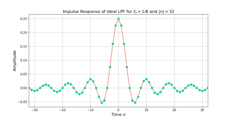
(10) ![\begin{equation*}\begin{split}h[n] & = \frac{1}{\pi n} \sin \left( 2 \pi f_n n \right) \\& = \frac{2 f_n}{2 f_n \pi n} \left( 2 \pi f_n n \right) \\& = 2 f_n \text{sinc} \left( 2 f_n n \right) \\\end{split}\end{equation*}](https://www.wavewalkerdsp.com/wp-content/ql-cache/quicklatex.com-2b3866dc14927abe96bfef70840997b6_l3.png "Rendered by QuickLaTeX.com")
The impulse response from (10) is given in Figure 2.