Wave Walker DSP

DSP Algorithms for RF Systems

Brand New Book!

DSP for Beginners: Simple Explanations for Complex Numbers! The second edition includes a new chapter on complex sinusoids.

Building a PSK and QAM Modulator in Python

June 8, 2022

Introduction

Taking an equation in a book and implementing it in hardware or software is hard. In this blog post I’ll show you how to interpret the equation for a PSK and QAM modulator and translate it into Python code.

Be sure to check out PySDR for another perspective on modulation!

Modulation

Single carrier modulators typically (but not always) involve the following operations:

Generating a data symbol or baud
Pulse shaping
Upconverting to pass-band

The next section describes common types of modulation schemes, or constellations, used for creating data symbols.

BPSK, QPSK, PSK and QAM

Binary Phase Shift Keying (BPSK) is one of the most fundamental modulation schemes for wireless communication. BPSK is characterized by two symbols, +1 and -1.

Where BPSK has two symbols, Quadrature Phase Shift Keying (QPSK) has four symbols. The symbols for QPSK are typically represented as

(1) $\begin{equation*}\frac{\sqrt{2}}{2}\left( 1 + j\right), \frac{\sqrt{2}}{2}\left( 1 - j\right), \frac{\sqrt{2}}{2}\left( -1 + j\right), \frac{\sqrt{2}}{2}\left( -1 - j\right).\end{equation*}$

Phase Shift Keying (PSK) is a modulation whose symbols are only along the unit circle. An example is 8-PSK, represented by

(2) $\begin{equation*}e^{j2\pi m / 8}, ~ m = \{0, 1, 2, \dots, 7\}.\end{equation*}$

BPSK can be considered 2-PSK and QPSK can be considered 4-PSK.

Quadrature Amplitude Modulation (QAM) is typically represents square or near-square modulations. An example is 16-QAM, whose real symbols are

(3) $\begin{equation*}-1, -1/3, 1/3, 1\end{equation*}$

and whose imaginary symbols are

(4) $\begin{equation*}-j, -j/3, j/3, j.\end{equation*}$

QPSK can be interpreted as 4-QAM.

The modulations of BPSK, QPSK, PSK and QAM are all tightly related and only differ by the number of constellation points and their location in the complex plane.

Pulse Shaping

A pulse shape is applied to data symbols in order to be good spectral neighbor, meaning the power in the sidelobes of a transmission needs to be minimized such that other transmitters can exist in the adjacent spectrum.

You may have noticed that FM radio stations are not directly next to one another on the dial, this is because guard bands are needed to minimize the adjacent channel interference.

An example of a pulse shape is the square-root raised cosine filter.

Upconversion

Upconversion, or frequency-mixing, is the process of translating a baseband signal up to a passband frequency. Upconversion is accomplished by multiplying the pulse shaped symbols by a complex exponential.

Textbook Equation

The following analysis uses QAM as the example signal. However, since BPSK, QPSK, PSK and QAM are all closely related the analysis will also apply to these modulations.

Proakis uses the following equation for QAM [proakis2001, p.174]:

(5) $\begin{equation*}s_{m}(t) = \text{RE}\left\{ (A_{mc} + j A_{ms}) g(t) e^{j2\pi f_{c}t} \right\}.\end{equation*}$

Let’s break down (5):

$s_{m}(t)$ is the result of modulating symbol m at time t
the real symbols are $A_{mc}$
the imaginary symbols are $j A_{ms}$
the pulse shape is $g(t)$
the upconversion is $e^{j2\pi f_{c} t$
the real component is taken through RE{ }

The next section will simplify the equation so it is easier to understand and translate into software.

Simplifying the Textbook Equation

Where (5) performs the upconversion to real pass-band, we will use a simplified representation by staying at complex baseband. This is accomplished by removing the upconversion step through setting $f_c = 0$ and removing the real operator RE{ },

(6) $\begin{equation*} s_{bb,m}(t) = (A_{mc} + j A_{ms}) g(t) \end{equation*}$

where $s_{bb,m}(t)$

is the complex baseband signal for symbol m. Further simplify by substituting

(7) $\begin{equation*}A_{m} = A_{mc} + j A_{ms}\end{equation*}$

where $A_{m}$

is the complex symbol to be modulated. The baseband signal is now written as

(8) $\begin{equation*}s_{bb,m}(t) = A_m g(t).\end{equation*}$

Since the signal is being generated digitally (8) needs to be sampled. The signal is sampled by substituting

(9) $\begin{equation*} t = n T_s, \end{equation*}$

where $T_s$

is the sampling period, resulting in

(10) $\begin{equation*}\begin{split}s_{bb,m}[n] & = s_{bb}(n T_s)\\& = A_{m} g(n T_s) \\& = A_{m} g[n].\end{split}\end{equation*}$

Equation (10) shows the $m^{th}$

complex symbol $A_m$

being pulse shaped by $g[n]$

. One modification (and a deviation from (5)) is the incorporation of a time delay such that the m+1 symbol occurs later in time than the m symbol,

(11) $\begin{equation*}s_{bb,m}[n] =A_{m} g[n-mN]\end{equation*}$

where N is the symbol period in samples. Equation (10) is rewritten as a summation over all symbols,

(12) $\begin{equation*} s_{bb}[n] = \sum_{m} A_{m} g[n-mN]. \end{equation*}$

Analyzing the Modulation Equation

Let’s define $g[n]$ to make analysis of (12) easier to understand.

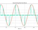
A simple (but impractical) pulse shape filter is the rectangular pulse shape, sometimes referred to as the boxcar window. The rectangular pulse shape uses all 1’s for N samples. This example rectangular pulse shape is chose to be of length $N = 4$ . The pulse shaping filter can then be written as

(13) $\begin{equation*}g[n] =\begin{cases}1, & 0 \le n \le 3 \\0, & \text{otherwise}.\end{cases}\end{equation*}$

Example samples of the modulated signal (12) can then be written as

(14) $\begin{equation*}A_{0}, A_{0}, A_{0}, A_{0}, A_{1}, A_{1}, A_{1}, A_{1}, A_{2}, A_{2}, A_{2}, A_{2}, \dots ~.\end{equation*}$

BPSK uses symbols of +1 and -1 and therefore an example of (14) could be written as

(15) $\begin{equation*}1, 1, 1, 1, -1, -1, -1, -1, 1, 1, 1, 1, \dots ~.\end{equation*}$

PSK and QAM Modulator Python Code

The modulator code in Python has to generate the sequence (14). There are many ways to do this in Python, including some that are more efficient, but this an illustrative example.

Import NumPy:

import numpy as np

Create the QPSK symbol map:

QPSKMapper = (np.sqrt(2) / 2) * np.array([1+1j, 1–1j, –1+1j, –1–1j])

Randomly generate some QPSK symbols:

ns = 16
mapIndex = np.random.randint(0, len(QPSKMapper), ns)
QPSKSymbols = QPSKMapper[mapIndex]

Define the samples per symbol, which is also the pulse shaping filter length:

SPS = 4

Upsample the symbols:

QPSKSymbolsUpsampled = np.zeros(ns*SPS,dtype=complex)
QPSKSymbolsUpsampled[::SPS] = QPSKSymbols

Define the pulse shaping filter:

pulseShape = np.ones(SPS)

Apply the pulse shaping filter:

QPSKSignal = np.convolve(QPSKSymbolsUpsampled,pulseShape)

The signal is now QPSK modulated! Other modulations such as PSK and QAM can be used by changing the QPSKMapper variable to include the desired constellation points.

Conclusion

This blog post started with a continuous-time equation for QAM and then simplified it into a discrete-time complex baseband signal. The equation was analyzed and simplified, and then used to create Python code for modulating QPSK, PSK and QAM signals.

2 Responses

Qasim says:

November 12, 2022 at 12:08 am

Hi Matt.
I saw your excellent website. Congratulations! One question: what is your complete process of rendering the image from production to web display? I am asking this question because your png images look crisper than most other png images on the web (they fade in quality for high resolution display). Thanks.

Reply
1. WaveWalkerDSP says:
  
  November 12, 2022 at 8:08 am
  
  Thank you!
  
  I generate them using Matplotlib within Python and save them as .png files using the savefig() call. I upload the raw .png files which are then compressed automatically using the EWWW image optimizer plugin.
  
  Hope this helps!
  
  Reply