Wave Walker DSP

DSP Algorithms for RF Systems

Buy the Book!

DSP for Beginners: Simple Explanations for Complex Numbers! The second edition includes a new chapter on complex sinusoids.

Single Pole IIR Filter: Substitute for Moving Average Filter

August 10, 2022

Introduction

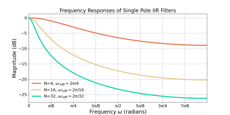
The single pole IIR filter is incredibly efficient and can be a great stand-in for a moving average filter! In this blog I describe how to derive the 3 dB bandwidth of the IIR filter to be equivalent to a moving average filter by designing the $\alpha$ weight. The design process builds on the IIR analysis from this DSP Stack Exchange question and my previous blog post.

Single Pole IIR

The impulse response of the single pole IIR filter is

(1) $\begin{equation*}y[n] = \alpha x[n] + (1-\alpha) y[n-1]\end{equation*}$

which can also be written as

(2) $\begin{equation*}y[n] = \alpha x[n] + \beta y[n-1]\end{equation*}$

where

(3) $\begin{equation*}\beta = 1-\alpha.\end{equation*}$

The magnitude of the frequency response of a single pole IIR filter is given by

(4) $\begin{equation*}\left|H\left(e^{j\omega}\right)\right| = \frac{\alpha}{\sqrt{\left(1 - \beta e^{-j\omega}\right)\left(1 - \beta e^{j\omega}\right)}},\end{equation*}$

where the magnitude-squared is

(5) $\begin{equation*}\left|H\left(e^{j\omega}\right)\right|^2 = \frac{\alpha^2}{\left(1 - \beta e^{-j\omega}\right)\left(1 - \beta e^{j\omega}\right)}.\end{equation*}$

Setting up the Design Problem

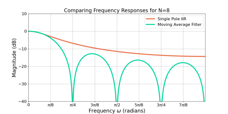
A previous blog post demonstrated how the 3 dB bandwidth of a moving average filter of length N can be approximated by

(6) $\begin{equation*}\omega_{3dB} = \pi/N.\end{equation*}$

The goal is to find the value $\alpha$ from (1) such that the 3 dB cutoff frequency of (5) is $\pi/N$ .

IIR Filter Design Equation

The 3 dB cutoff corresponds to a magnitude-squared of 1/2. The design equation is therefore

(7) $\begin{equation*}\frac{\alpha^2}{\left(1 - \beta e^{-j\omega}\right)\left(1 - \beta e^{j\omega}\right)} = \frac{1}{2}.\end{equation*}$

Multiplying the complex exponential terms,

(8) $\begin{equation*}\frac{\alpha^2}{1 + \beta^2 - \beta e^{j\omega} - \beta e^{-j\omega}} = \frac{1}{2},\end{equation*}$

which is simplified as

(9) $\begin{equation*}\frac{\alpha^2}{1 + \beta^2 - \beta \left( e^{j\omega} + e^{-j\omega}\right)} = \frac{1}{2}.\end{equation*}$

The complex exponentials can be written in terms of cosine,

(10) $\begin{equation*}2\cos\left( \omega \right) = e^{j\omega} + e^{-j\omega}.\end{equation*}$

Substituting (10) into (9),

(11) $\begin{equation*}\frac{\alpha^2}{1 + \beta^2 - 2\beta \cos\left( \omega \right)} = \frac{1}{2}.\end{equation*}$

Multiplying the terms of (11) results in

(12) $\begin{equation*}\begin{split}2\alpha^2 & = 1 + \beta^2 - 2 \beta \cos(\omega)\\0 & = - 2\alpha^2+ 1 + \beta^2 - 2 \beta \cos(\omega)\\\end{split}\end{equation*}$

Substituting $\beta = 1-\alpha$ ,

(13) $\begin{equation*}\begin{split}0 & = -2\alpha^2 +1 + (1-\alpha)^2 - 2 (1-\alpha)\cos\left( \omega \right) \\0 & = -2\alpha^2 +1 + (1+\alpha^2-2\alpha) - 2 (1-\alpha)\cos\left( \omega \right) \\0 & = -\alpha^2 + 2\alpha\left(\cos\left( \omega \right)-1\right) + 2\left(1-\cos\left( \omega \right) \right) \\0 & = \alpha^2 + 2\alpha\left( 1 - \cos\left( \omega \right)\right) -2\left(1-\cos\left(\omega\right)\right).\end{split}\end{equation*}$

Solving with the Quadratic Equation

The design equation (13) can be solved for $\alpha$ using the quadratic equation,

(14) $\begin{equation*}\alpha = \frac{- b \pm \sqrt{b^2-4ac}}{2a}\end{equation*}$

where

(15) $\begin{equation*}a = 1,\end{equation*}$

(16) $\begin{equation*}b = 2\left( 1-\cos\left( \omega \right)\right),\end{equation*}$

(17) $\begin{equation*}c = -2\left(1-\cos\left( \omega \right)\right).\end{equation*}$

Substituting (15), (16) and (17) into (14),

(18) $\begin{equation*}\alpha = \frac{- 2\left( 1-\cos\left( \omega \right)\right) \pm \sqrt{\left(2\left( 1-\cos\left( \omega \right)\right)\right)^2-4\left(-2\left(1-\cos\left( \omega \right)\right)\right)}}{2}.\end{equation*}$

Simplifying (18),

(19) $\begin{equation*}\begin{split}\alpha & = \frac{- 2\left( 1-\cos\left( \omega \right)\right) \pm \sqrt{4\left( 1-\cos\left( \omega \right)\right)^2 +8\left(1-\cos\left( \omega \right)\right)}}{2} \\& = \frac{- 2\left( 1-\cos\left( \omega \right)\right) \pm 2\sqrt{\left( 1-\cos\left( \omega \right)\right)^2 +2\left(1-\cos\left( \omega \right)\right)}}{2} \\& = -\left( 1-\cos\left( \omega \right)\right) \pm \sqrt{\left( 1-\cos\left( \omega \right)\right)^2 +2\left(1-\cos\left( \omega \right)\right)} \\& = \cos\left( \omega \right)-1 \pm \sqrt{1-2\cos\left( \omega \right)+\cos^2\left(\omega\right) +2-2\cos\left( \omega \right)} \\& = \cos\left( \omega \right)-1 \pm \sqrt{3-4\cos\left( \omega \right)+\cos^2\left(\omega\right)} \\\end{split}\end{equation*}$

Picking the Alpha Value

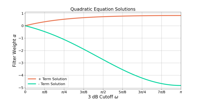
The design equation in (19) has two solutions due to the $\pm$ term. Figure 1 shows the two solutions for $0 \le \omega \le \pi$ .

The + from the $\pm$ is chosen from (19) to select the positive coefficient, therefore the final design equation is

(20) $\begin{equation*}\alpha = \cos\left( \omega \right)-1 + \sqrt{3-4\cos\left( \omega \right)+\cos^2\left(\omega\right)}.\end{equation*}$

To design a high pass filter (HPF), choose the – term in the $\pm$ from (19).

Approximating the Moving Average Filter

The 3 dB cutoff for a length N moving average filter from (6) is substituted into the design equation (20) and the magnitude of the frequency response is plotted in Figure 2 for multiple values of N.

Comparison to Moving Average Filter

Figure 2 shows that increasing the filter cutoff frequency also reduces the sidelobe attenuation. Although the single pole IIR filter uses less computation than a moving average filter, it also has lower attenuation of out of band frequency content. Figure 3 shows that the single pole IIR filter approaches the response of the moving average filter for N=8 but with about 4 dB worse attenuation.

Conclusion

The single pole IIR filter is a great substitute to the moving average filter! The substitution trades slightly worse sidelobe attenuation for a decrease in computation needed to implement the filter. This blog post described how to design the single pole IIR filter weight to approximate the frequency response of a moving average filter.