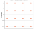
![Figure 3: The complex sinusoid e(j2 pi (2/4) n) only contains energy at X[2].](https://www.wavewalkerdsp.com/wp-content/uploads/wordpress-popular-posts/8136-featured-125x100.png)
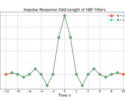
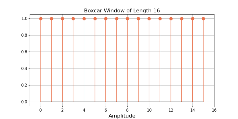
![\begin{equation*}h[n] = \begin{cases}1, & 0 \le n \le N-1 \\0, & \text{otherwise}.\end{cases}\end{equation*}](https://www.wavewalkerdsp.com/wp-content/ql-cache/quicklatex.com-27c5cdc5cf8357ef647888d1b84b5bfd_l3.png "Rendered by QuickLaTeX.com")
Since (1) is discrete-time the Discrete-Time Fourier Transform (DTFT) must be taken.
The DTFT is defined as (reference)
(2) ![\begin{equation*}X\left(e^{j\omega}\right) = \sum_{n} x[n]e^{-j \omega n}.\end{equation*}](https://www.wavewalkerdsp.com/wp-content/ql-cache/quicklatex.com-88e45a2bc3da0d315e481b9239354d61_l3.png "Rendered by QuickLaTeX.com")
(3) ![\begin{equation*}\begin{split}H\left( e^{j\omega} \right) & = \sum_{n} h[n] e^{-j\omega n} \\& = \sum_{n=0}^{N-1} e^{-j\omega n}.\end{split}\end{equation*}](https://www.wavewalkerdsp.com/wp-content/ql-cache/quicklatex.com-496e9c57c6148dc58da0a8a162be2f6b_l3.png "Rendered by QuickLaTeX.com")
Equation (3) is now a finite geometric series. The sum of a finite geometric series
(4) 
can be written as (reference)
(5) 
Comparing (3) to (4), a = 1 and  . The summation from (5) can therefore be written as
(6) 
The magnitude-squared of (6) is given by
(7) 
Multiplying the terms from (7),
(8) 
Gathering like terms,
(9) 
The complex exponentials can be written in terms of cosine such that
(10) 
which can be simplified to:
(11) 
Equation (11) for N=16 is plotted in Figure 2. The computed magnitude is shown along side to show their equivalence and the correctness of the derivation.
