Wave Walker DSP

DSP Algorithms for RF Systems

Buy the Book!

DSP for Beginners: Simple Explanations for Complex Numbers! The second edition includes a new chapter on complex sinusoids.

Derivative Filter Impulse Response Derivation

November 24, 2021

Introduction

Sooner or later you’re going to have to apply a derivative to a discrete-time signal. An example would be building a derivative matched filter (DMF) for timing recovery [harris2021, p.490]. This brings us to our first piece of DSP Wisdom: If you need to do something in DSP it’s best to do it with a filter. So how do you build a derivative filter?

We’ll start with the derivation in continuous-time to make the math tractable then transform it into discrete-time. A follow-up post will discuss methods and alternatives for designing the derivative filter weights. Richard Lyons has a really great section on derivative filters in his textbook that is totally worth your time if you’re interested in more information on the topic [lyons2011, p.361].

Check out these other posts on filter design:

Continuous-Time Derivative Filter

The time-derivative of signal $x(t)$ can be written as the derivative of the inverse Fourier transform,

(1) $\begin{equation*}x'(t) = \frac{d}{dt} \left( \int_{-\infty}^{\infty} X(f) e^{j 2\pi f t} df \right).\end{equation*}$

Pulling the derivative $d/dt$ through the integral in (1) results in

(2) $\begin{equation*}x'(t) = \int_{-\infty}^{\infty} X(f) \frac{d}{dt} \left( e^{j2\pi f t} \right) df.\end{equation*}$

The derivative of the complex sinusoid can be written as

(3) $\begin{equation*}\frac{d}{dt} e^{j 2\pi f t} = j 2\pi f \cdot e^{j 2\pi f t}.\end{equation*}$

Substituting the derivative (3) into (2) can be written as

(4) $\begin{equation*}x'(t) = \int_{-\infty}^{\infty} j 2 \pi f X(f) e^{j2\pi f t} df.\end{equation*}$

The signal derivative (4) can be rewritten using the inverse Fourier transform operator $\mathcal{F}^{-1} \{ \cdot \}$ such that

(5) $\begin{equation*}x'(t) = \mathcal{F}^{-1} \{ j 2\pi f X(f) \}.\end{equation*}$

A frequency-domain derivative filter is defined as

(6) $\begin{equation*}H(f) = j 2\pi f\end{equation*}$

such that (5) is

(7) $\begin{equation*}x'(t) = \mathcal{F}^{-1} \{ H(f) \cdot X(f) \}.\end{equation*}$

The product of two frequency-responses A(f) and B(f) are related through the Fourier transform to the convolution $\ast$ of their impulse-responses a(t) and b(t)

(8) $\begin{equation*}\begin{split}\mathcal{F}^{-1} \{A(f) \cdot B(f)\} & = \mathcal{F}^{-1} \{ A(f) \} \ast \mathcal{F}^{-1} \{ B(f) \} \\& = a(t) \ast b(t).\end{split}\end{equation*}$

The signal derivative (7) can therefore be written as the convolution of two impulse-responses, the signal x(t) and the derivative filter h(t),

(9) $\begin{equation*}\begin{split}x'(t) & = \mathcal{F}^{-1} \{ H(f) \} \ast \mathcal{F}^{-1} \{ X(f) \} \\& = h(t) \ast x(t).\end{split}\end{equation*}$

The impulse response of the derivative filter is defined through the inverse Fourier transform

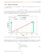
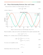
(10) $\begin{equation*}\begin{split}h(t) & = \mathcal{F}^{-1} \{H(f)\} \\& = \mathcal{F}^{-1} \{ j 2\pi f \}.\end{split}\end{equation*}$

Figure 1 is a 3D plot of the frequency-response H(f) for some values of f where

(11) $\begin{equation*}\text{RE} \{ H(f) \} = 0,\end{equation*}$

(12) $\begin{equation*}\text{IM} \{ H(f) \} = j2\pi f.\end{equation*}$

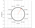
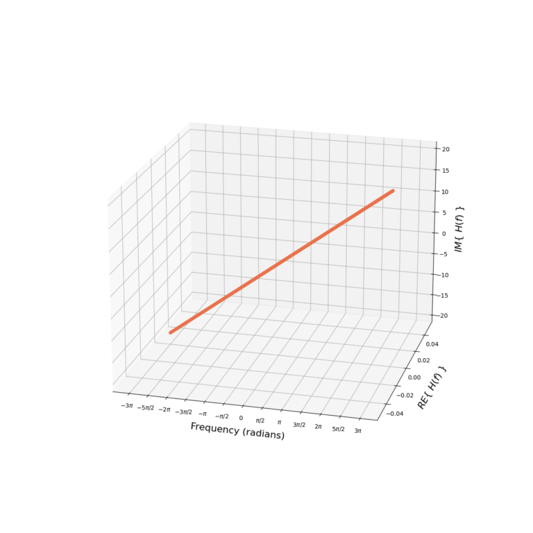
The magnitude $|H(f)|$ and phase $\sphericalangle{H(f)}$ of the derivative filter are given in Figure 2.

Transforming into a Discrete-Time Frequency Response

A discrete-time implementation of $H(f) = j2\pi f$ from (6) is created by truncating the frequency response. Where H(f) is defined over $-\infty < f < \infty$ the discrete-time Fourier transform (DTFT) is defined by

(13) $\begin{equation*}H(e^{j \omega}) = j \omega\end{equation*}$

where

(14) $\begin{equation*}\omega = 2\pi \frac{f}{f_s}.\end{equation*}$

The sampling rate defines the amount of truncation such that $H(e^{j\omega})$ is defined over $-\pi \le \omega \le \pi$ or equivalently $-f_s/2 \le f \le f_s/2$ .

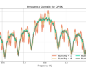
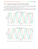
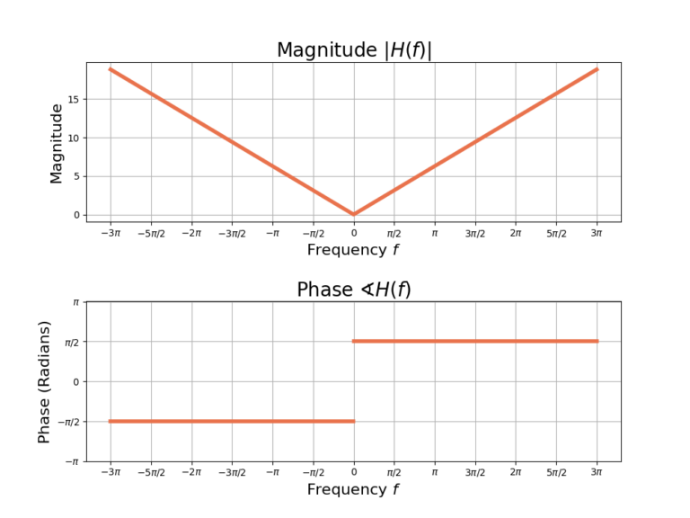
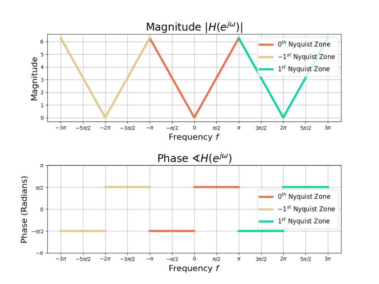
Figure 3 gives the frequency-response $H(e^{j\omega})$ for the discrete-time derivative filter. The frequency-response is periodic in $2\pi$ and three repetitions are shown, denoted as Nyquist zones -1, 0 and 1. Figure 4 is the magnitude $|H(f)|$ and phase $\sphericalangle{H(f)}$ which also shows three Nyquist zones.

Discrete-Time Derivative Filter

The continuous-time frequency-response H(f) in (6) was mapped into discrete-time $H(e^{j\omega})$ in (13). The inverse DTFT is used to transform $H(e^{j\omega})$ into the impulse-response h[n] where the inverse DTFT is given by [oppenheim1999, p.48]

(15) $\begin{equation*}h[n] = \frac{1}{2\pi} \int_{-\pi}^{\pi} H(e^{j\omega}) e^{j\omega n} ~ d\omega.\end{equation*}$

Substituting $H(e^{j\omega}) = j\omega$ from (13) into (15) results in

(16) $\begin{equation*}h[n] = \frac{1}{2\pi} \int_{-\pi}^{\pi} j \omega e^{j\omega n} ~ d\omega.\end{equation*}$

The inverse DTFT integral (16) can be solved through the use of integration by parts. Define u and v according to

(17) $\begin{equation*}\begin{split}u & = \omega \\du & = d\omega \\v & = e^{j\omega n}/(jn) \\dv & = e^{j\omega n}.\end{split}\end{equation*}$

Integration by parts of the inverse DTFT integral (16) is defined as

(18) $\begin{equation*}h[n] = \frac{j}{2\pi} \left( u \cdot v \Big|_{-\pi}^{\pi} - \int_{-\pi}^{\pi} v ~ du \right)\end{equation*}$

and substituting (17) into (18) results in

(19) $\begin{equation*}\begin{split}h[n] & = \frac{j}{2\pi} \left( \frac{\omega}{jn} e^{j\omega n} \Big|_{-\pi}^{\pi} - \int_{-\pi}^{\pi} \frac{1}{jn} e^{j\omega n} d\omega \right) \\& = \frac{\omega}{2\pi n} e^{j\omega n} \Big|_{-\pi}^{\pi} - \frac{1}{2\pi n} \int_{-\pi}^{\pi} e^{j\omega n} d\omega. \end{split}\end{equation*}$

Evaluating the Integral (Part 1)

The first part of (19) can be simplified as

(20) $\begin{equation*}\begin{split}\frac{\omega}{2\pi n} e^{j\omega n} \Big|_{-\pi}^{\pi} & = \frac{1}{2\pi n} \left( \pi e^{j\pi n} - (-\pi)e^{-j\pi n} \right) \\& = \frac{1}{2n}\left( e^{j\pi n} + e^{-j\pi n} \right).\end{split}\end{equation*}$

Equation (20) can be simplified to

(21) $\begin{equation*}\frac{1}{n} \left( \frac{1}{2} \left( e^{j\pi n} + e^{-j\pi n} \right) \right) = \frac{1}{n} \text{cos}(\pi n).\end{equation*}$

The term $\cos(\pi n)$ can be written as

(22) $\begin{equation*}\text{cos}(\pi n) = (-1)^n\end{equation*}$

for all n, however evaluating (21) at n=0 must be done through L’Hopital’s rule,

(23) $\begin{equation*}\begin{split}\lim_{n\rightarrow 0} \frac{ \frac{\partial }{\partial n} \text{cos}\left( \pi n \right) } { \frac{\partial}{\partial n} \pi n } & = \lim_{n\rightarrow 0} \frac{ -\text{sin}\left( \pi n \right) } { \pi } \\& = \frac{0}{\pi} \\& = 0.\end{split}\end{equation*}$

Using (23) and (22), equation (21) is written as

(24) $\begin{equation*}\frac{1}{n} \text{cos}(\pi n) =\begin{cases}0, & n = 0 \\\frac{(-1)^n}{n}, \text{otherwise}.\end{cases}\end{equation*}$

Evaluating The Integral (Part 2)

The second part of (19) is

(25) $\begin{equation*}\begin{split}- \frac{1}{2\pi n} \int_{-\pi}^{\pi} e^{j\omega n} d\omega \right) & = -\frac{1}{j2\pi n^2} \left( e^{j\pi n} - e^{-j\pi n} \right) \\& = -\frac{1}{\pi n^2} \left( \frac{e^{j\pi n} - e^{-j\pi n}}{2j} \right)\end{split}\end{equation*}$

which can be simplified by a trigonometric identity to

(26) $\begin{equation*}-\frac{1}{\pi n^2} \left( \frac{e^{j\pi n} - e^{-j\pi n}}{2j} \right) = -\frac{1}{\pi n^2} sin(\pi n).\end{equation*}$

The term $\sin(\pi n)$ can be reduced to

(27) $\begin{equation*}sin(\pi n) = 0\end{equation*}$

for all n, however evaluating (26) at n=0 must be done through L’Hopital’s rule. Applying L’Hopital’s Rule on (26) is

(28) $\begin{equation*}\lim_{n\rightarrow 0} \frac{ -\frac{\partial}{\partial n} \text{sin}(\pi n) }{ \frac{\partial}{\partial n} \pi n^2 } = \lim_{n\rightarrow 0} \frac{ -\text{cos}(\pi n) } {2\pi n}\end{equation*}$

which still cannot be evaluated at n=0 and therefore the rule is applied once more,

(29) $\begin{equation*}\begin{split}\lim_{n\rightarrow 0} \frac{ -\frac{\partial}{\partial n} \text{cos}(\pi n) }{ \frac{\partial}{\partial n} 2 \pi n } & = \lim_{n\rightarrow 0} \frac{ -\text{cos}(\pi n) } {2\pi n} \\& = \lim_{n\rightarrow 0} \frac{ sin(\pi n) }{ 2 \pi } \\& = \frac{0}{2\pi} \\& = 0.\end{split}\end{equation*}$

Derivative Filter Impulse Response

The impulse-response of the derivative filter h[n] (19) is the summation of the two terms (24) and (29)

(30) $\begin{equation*}h[n] = \begin{cases}\frac{(-1)}{n}, & n \neq 0 \\0, & n = 0\end{cases}\end{equation*}$

which is an infinitely long filter. A truncated impulse response from (30) is given in Figure 5 and the magnitude and phase of the frequency response in Figure 6.

Conclusion

A derivative filter is a useful tool to have in your DSP kit. The derivation starts with a time-derivative of the frequency-response which results in the product of two frequency responses, or equivalently the convolution of two impulse-responses. Applying the inverse DTFT results in an infinitely long impulse response for the derivative filter.

Figure 6 shows a different magnitude and phase than the ideal plots in Figure 2. Be on the look out for part 2 in which the differences will be discussed in detail and methods will be given for designing derivative filter weights.