![Figure 1: The weights of the partitioned half band filter hA[n] and hB[n].](https://www.wavewalkerdsp.com/wp-content/uploads/wordpress-popular-posts/2226-featured-125x100.png)
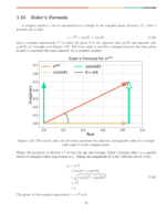
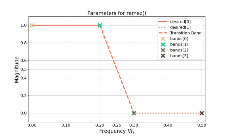
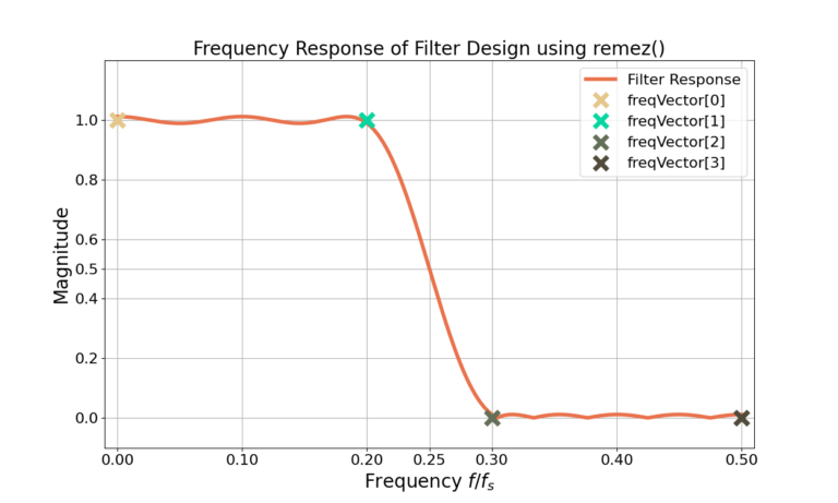
As expected the designed magnitude response in Figure 3 goes approximately through the locations defined by both freqVec and ampVec. The magnitude of a frequency response is typically viewed in decibels, through the relationship
(1) ![\begin{equation*}10\text{log}_{10} ( |X[k]|^2 ) = 20\text{log}_{10}( |X[k]| ),\end{equation*}](https://www.wavewalkerdsp.com/wp-content/ql-cache/quicklatex.com-f189235ed694823f1a8404274e5d70e0_l3.png "Rendered by QuickLaTeX.com")
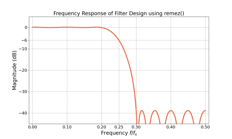
where ![X[k]](https://www.wavewalkerdsp.com/wp-content/ql-cache/quicklatex.com-bb570fd2ccdd02a3f23849c4ef80a7b8_l3.png "Rendered by QuickLaTeX.com") is the frequency response. Note that when the magnitude in the frequency domain is displayed it is most commonly the magnitude-squared as in (1), as in Figure 4.
is the frequency response. Note that when the magnitude in the frequency domain is displayed it is most commonly the magnitude-squared as in (1), as in Figure 4.
fred harris’ filter length approximation [harris2021, p.59] is
(2) 
where  is the transition bandwidth,
  is the sampling frequency and
  is the sidelobe attenuation in dB. The frequencies and can be in any units as long as they are consistent.
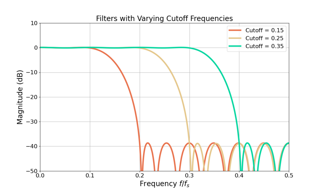
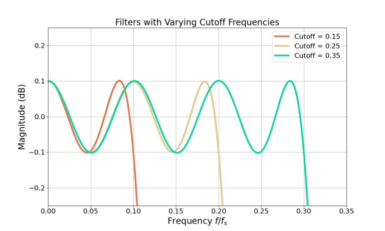
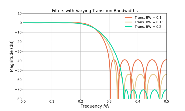
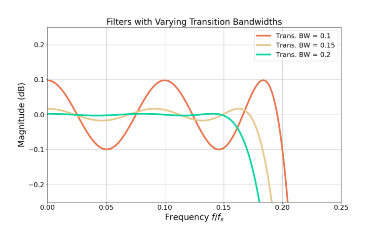
The approximation in (2) shows that changes to the transition bandwidth will directly impact the sidelobe attenuation when the filter length is held constant. However the cut-off frequency has no impact which reinforces the earlier filters from Figures 4 – 8.
Using the parameters from Figure 7, =39 and  , the filter length for a transition bandwidth of
  is approximated to be
(3) 
Similarly from Figure 7, the second filter with  and
and  gives a filter length approximation of
(4) 
and the second filter with  and
and  gives a filter length approximation of
(5) 
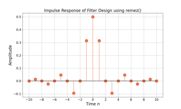
The filter lengths are not exact but are reasonably close to the length L=21 the filter was designed with. It is typical for filter design to be an iterative “guess and check” process until the exact desired weights or frequency response is obtained.
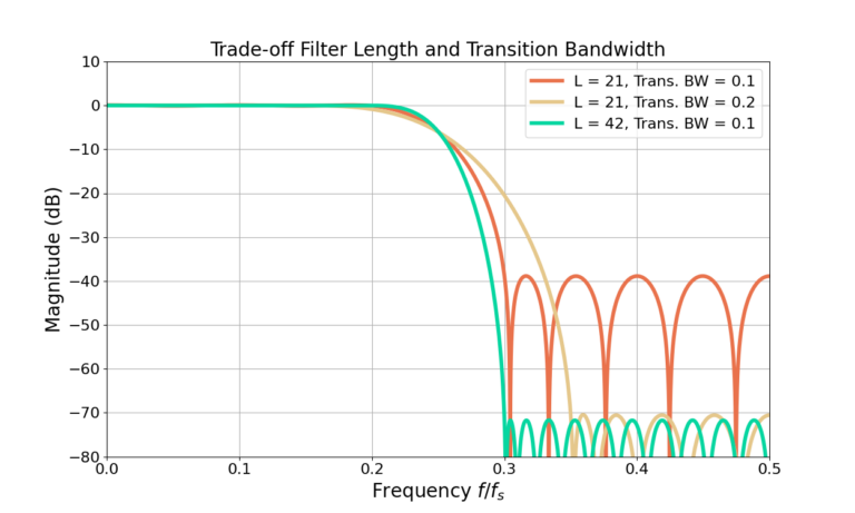
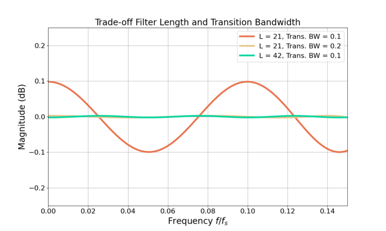
A great filter will have:
- a short length to reduce computation,
- a small transition band to maximize the amount of pass-band and stop-band,
- small pass-band ripple and large stop-band attenuation.
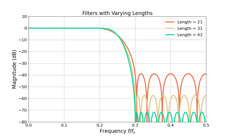
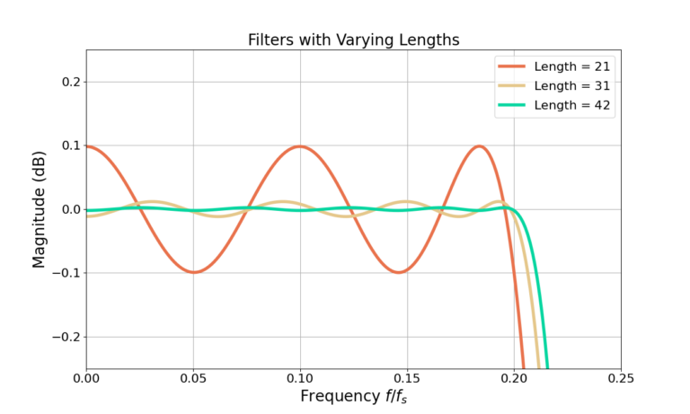
However, due to (2) a filter cannot have all three of these attributes and design trade-offs must be made. Figure 11 and Figure 12 show the example filter with L=21 and which has sidelobes at -39 dB and a pass-band ripple of 0.2 dB. The two other filters increase the sidelobe attenuation to about -70 dB by two different methods: doubling the transition bandwidth and doubling the filter length.