![A BPSK signal s[n], real Gaussian noise w[n], and the received signal x[n] = s[n] + w[n] for SNR = 20 dB](https://www.wavewalkerdsp.com/wp-content/uploads/wordpress-popular-posts/15621-featured-125x100.png)

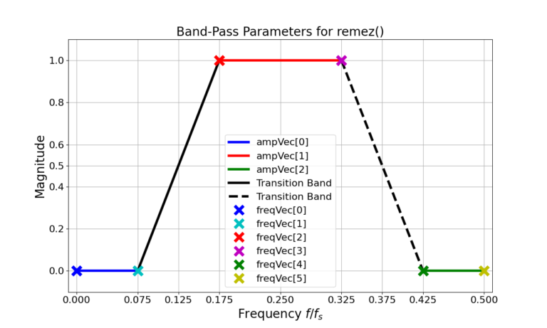
An example pass-band filter can be designed with remez() by
import scipy.signal
fCenter = 0.25
passbandWidth = 0.25
transBandBPF = 0.2
fPassLeft = fCenter - (passbandWidth/2)
fPassRight = fCenter + (passbandWidth/2)
fStopLeft = fPassLeft - (transBandBPF/2)
fStopRight = fPassRight + (transBandBPF/2)
fVec = [0, fStopLeft, fPassLeft, fPassRight, fStopRight, 0.5]
aVec = [0, 1, 0]
BPFRemez = scipy.signal.remez(filterLength,fVec,aVec)
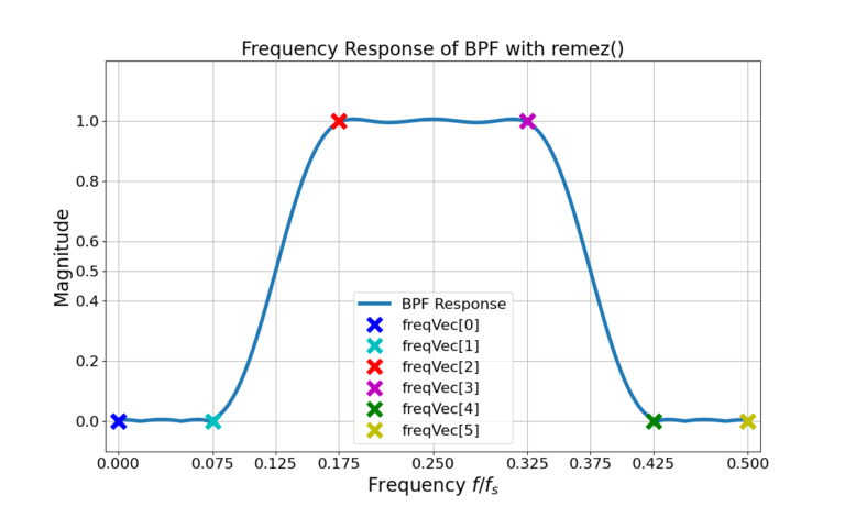
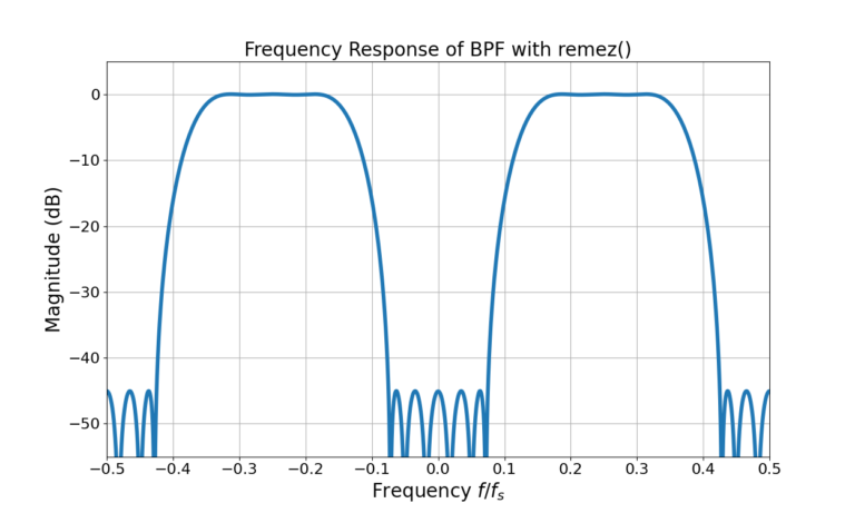
Figure 1 displays the design parameters of the BPF and the desired shape of the magnitude of the frequency response, Figure 2 gives the actual frequency response in linear units. A BPF has two transition bands (Figure 1 and Figure 2), one to the left and one to the right of the passband. Therefore the transition bandwidth of 0.2 is divided to both, 0.1 to the left and 0.1 to the right.
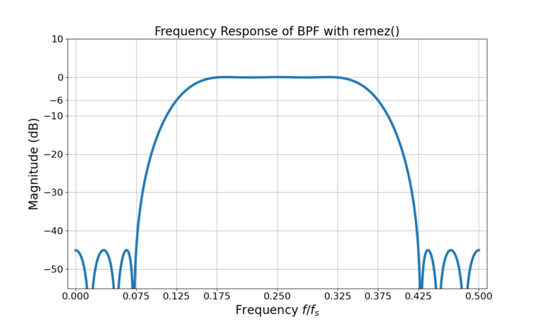
Figure 3 gives the magnitude of the frequency response for the BPF in dB and Figure 4 displays the double sided spectrum from  to
to  , or
, or  to
to  in radians.
Similar to the process from the high-pass filter design blog an LPF is designed and then upconverted to band-pass. The LPF is designed with
import scipy.signal
filterLength = 21
cutoffLPF = 0.125
transBand = 0.1
fPassLPF = cutoffLPF - (transBand/2)
fStopLPF = cutoffLPF + (transBand/2)
fVec = [0, fPassLPF, fStopLPF, 0.5]
aVec = [1, 0]
LPFRemez = scipy.signal.remez(filterLength,fVec,aVec)
The filter weights are then upconverted to  or
or  in radians,
(1) ![\begin{equation*}h_{BPF}[n] = h_{LPF}[n] \cdot cos(\pi n/2).\end{equation*}](https://www.wavewalkerdsp.com/wp-content/ql-cache/quicklatex.com-49f19c19aa78ddc0af237c16d5c6ea59_l3.png "Rendered by QuickLaTeX.com")
Figure 6 gives the frequency responses for the BPF designed with Remez as well as the LPF upconverted to band-pass.
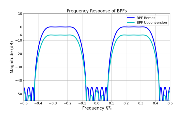
The first thing to note from Figure 6 is that the magnitude is 6 dB lower than the Remez version. Why?
Taking another look at the math, cosine can be expressed as the summation of two complex exponentials,
(2) 
(3) ![\begin{equation*}\begin{split}h_{BPF}[n] & = h_{LPF}[n] \cdot \frac{1}{2} \left( e^{j\pi n/2} + e^{-j \pi n/2} \right) \\& = \left( \frac{1}{2} h_{LPF}[n] \cdot e^{j\pi n/2} \right ) + \left( \frac{1}{2} h_{LPF}[n] \cdot e^{-j\pi n/2} \right ).\end{split}\end{equation*}](https://www.wavewalkerdsp.com/wp-content/ql-cache/quicklatex.com-6d72891abd56cf8bef2cd999b105bb88_l3.png "Rendered by QuickLaTeX.com")
The LPF is turned into two copies at different frequencies whose magnitude is divided by 1/2. Scaling the upconverted BPF by 2 accounts for the relative loss compared to the Remez design,
(4) ![\begin{equation*}h_{BPF}[n] = 2 \cdot h_{LPF}[n] \cdot cos(\pi n/2).\end{equation*}](https://www.wavewalkerdsp.com/wp-content/ql-cache/quicklatex.com-59a37d4a28ee358e6bbbf6026bf11f18_l3.png "Rendered by QuickLaTeX.com")
Figure 7 gives the frequency response for (4).
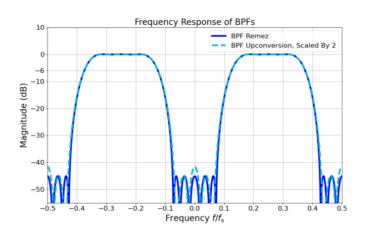
The scaling by 2 has matched the magnitude levels of the two filters in Figure 7 however the sidelobes now show a difference. The sidelobes are higher at  . Why?
The problem is ![h_{LPF}[n] \cdot e^{j\pi n/2}](https://www.wavewalkerdsp.com/wp-content/ql-cache/quicklatex.com-58b3a6945c9a6159f834501a725110d9_l3.png "Rendered by QuickLaTeX.com") and
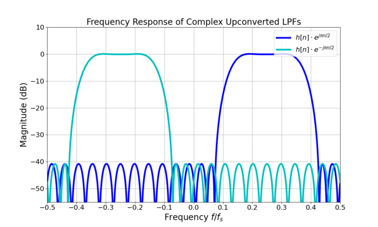
and ![h_{LPF}[n] \cdot e^{-j\pi n/2}](https://www.wavewalkerdsp.com/wp-content/ql-cache/quicklatex.com-c13460fdece1e57d7e73a332a60908a6_l3.png "Rendered by QuickLaTeX.com") interfere with one another in the frequency domain when they are summed. Figure 8 shows the two frequency responses of the complex upconversion to positive and negative frequencies of the BPF.
interfere with one another in the frequency domain when they are summed. Figure 8 shows the two frequency responses of the complex upconversion to positive and negative frequencies of the BPF.
Real signals have an evenly symmetric magnitude [oppenheim1999, p.56], that is
(5) 
Equation (5) is the reason why ![h_{LPF}[n] \cdot cos(\pi n/2)](https://www.wavewalkerdsp.com/wp-content/ql-cache/quicklatex.com-2d039927c9edbc4c4ad2b5ba5ac732b6_l3.png "Rendered by QuickLaTeX.com") has a passband in both the positive frequencies and negative frequencies. Such an even-symmetric respond may be acceptable when processing real signals but much of DSP is done at complex baseband and non-symmetric band-pass filters may be required in the case of channelizers, for selecting specific signals from a broad spectrum or applying a Hilbert transform [carrick2011].
has a passband in both the positive frequencies and negative frequencies. Such an even-symmetric respond may be acceptable when processing real signals but much of DSP is done at complex baseband and non-symmetric band-pass filters may be required in the case of channelizers, for selecting specific signals from a broad spectrum or applying a Hilbert transform [carrick2011].
Where ![h_{BPF}[n]](https://www.wavewalkerdsp.com/wp-content/ql-cache/quicklatex.com-33587ae0dac2c64249cf1cdcce13cffd_l3.png "Rendered by QuickLaTeX.com") in (4) uses real upconversion complex upconversion can be used to translate a LPF into complex band-pass. Rather than use a cosine to perform the upconversion, a complex-exponential will allow the selection of one of the two BPF responses as in Figure 8.
in (4) uses real upconversion complex upconversion can be used to translate a LPF into complex band-pass. Rather than use a cosine to perform the upconversion, a complex-exponential will allow the selection of one of the two BPF responses as in Figure 8.
The positive and negative frequency complex upconverted band-pass filter is given by
(6) ![\begin{equation*}h_{+BPF}[n] = h_{LPF}[n] \cdot e^{j \phi n}\end{equation*}](https://www.wavewalkerdsp.com/wp-content/ql-cache/quicklatex.com-6f52ec4d12980812ff20255ca81f905f_l3.png "Rendered by QuickLaTeX.com")
(7) ![\begin{equation*}h_{-BPF}[n] = h_{LPF}[n] \cdot e^{-j \phi n}\end{equation*}](https://www.wavewalkerdsp.com/wp-content/ql-cache/quicklatex.com-96feccdb57c90ed4260c422ea2bad9f2_l3.png "Rendered by QuickLaTeX.com")
where  and \(-\phi)\ is the center frequency of the band-pass filter. The filters can be upconverted using the following code:
import numpy as np
n = np.arange(-(filterLength-1)/2,(filterLength-1)/2+1)
BPFPosUpconvert = LPFRemez*np.exp(1j*2*np.pi*n*(1/4))
BPFNegUpconvert = LPFRemez*np.exp(-1j*2*np.pi*n*(1/4))
The downside of the complex upconversion is that the filter weights are transformed from real to complex and therefore the filter now requires complex multiplication to implement it which requires more operations.
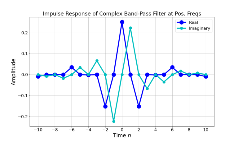
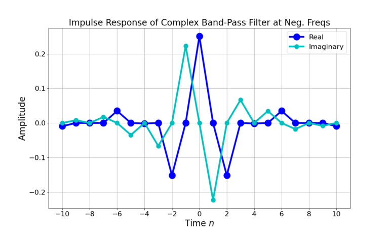
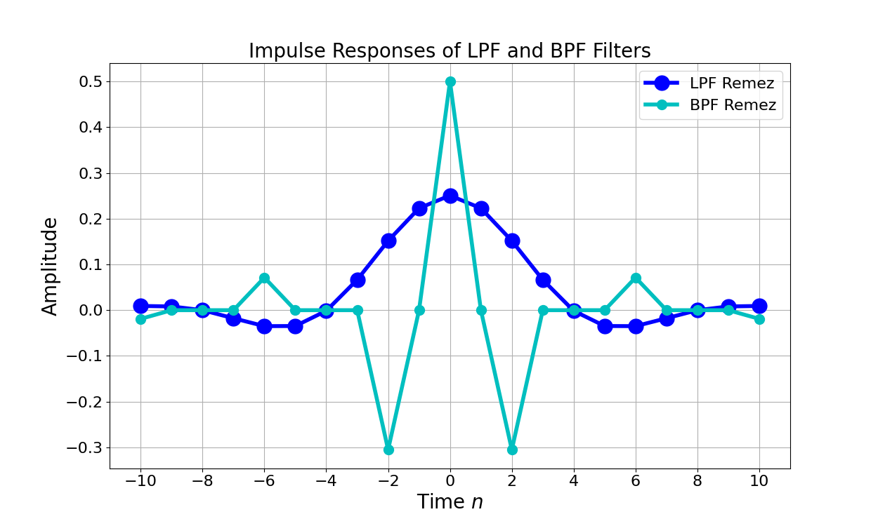
Figure 9 is the impulse response of the LPF being upconverted to complex pass-band at positive frequencies from (6) and Figure 10 is after being upconverted to negative frequencies from (7). Note that the imaginary portion of the impulse response is delayed with respect to the real for the positive frequency BPF in Figure 9. The real portion of the impulse response is delayed with respect to the imaginary in Figure 10 which is characteristic of a negative frequency sinusoid.