![Figure 1: The weights of the partitioned half band filter hA[n] and hB[n].](https://www.wavewalkerdsp.com/wp-content/uploads/wordpress-popular-posts/2226-featured-125x100.png)
![A BPSK signal s[n], real Gaussian noise w[n], and the received signal x[n] = s[n] + w[n] for SNR = 20 dB](https://www.wavewalkerdsp.com/wp-content/uploads/wordpress-popular-posts/15621-featured-125x100.png)
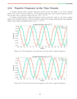
The mathematics of DSP and complex numbers can be confounding.
Understanding how  was difficult when I first started my DSP education and it’s still not something I fully grasp. When starting out in your DSP education sometimes it is enough to simply understanding how the tools and procedures are applied, rather than how they are derived.
Personally, early in my career I accepted the fact that is true and useful, along with a host of other equations. Over many years of experience in the classroom and in the laboratory I have build some intuition around the mathematics and can apply them appropriately. But it all started with understanding the mathematical rules of complex numbers.
More posts on complex numbers:


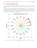
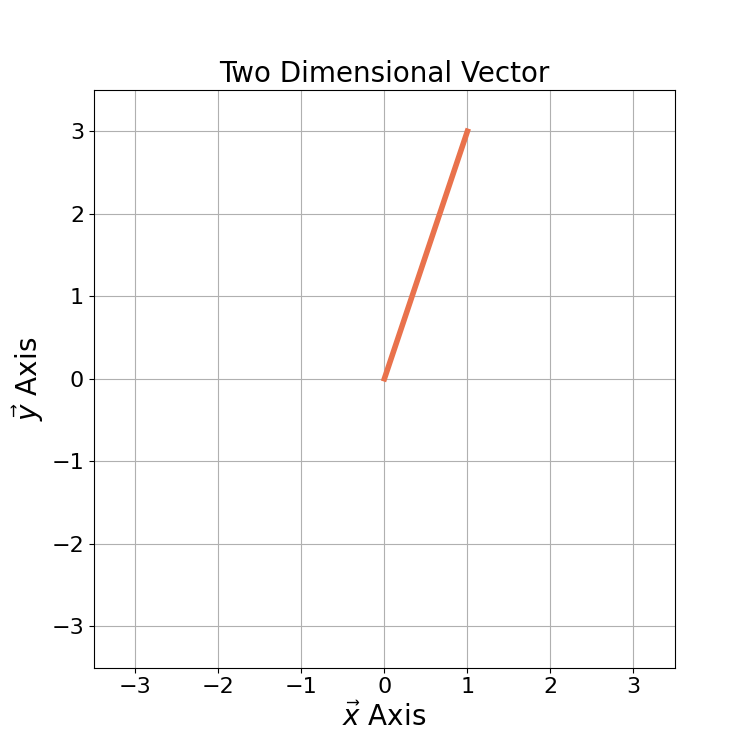
Cartesian form is one way to represent complex numbers in a form similar to two dimensional vectors. Cartesian form is the default representation used in computing systems. An example of a two dimensional vector  is given by
(7) 
where  and
and  are unit vectors. The values c and d are independent of one another because the two unit vectors and are orthogonal to one another. An example of a two-dimensional vector is given in Figure 1.
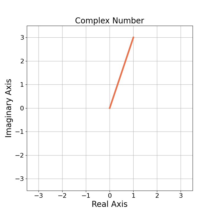
Complex numbers are similar to two-dimensional linear vectors but with additional mathematic relationships. Complex numbers are made of real and imaginary components. For the complex number c,
(8) 
a is the real component and b is the imaginary component. Where the unit vectors and are made explicit in (7), the unit vector for a is implied and the unit vector for b is j. Figure 2 gives an example of a complex number plotted in the complex domain.
The magnitude of a complex number is it’s length in the complex domain,
(9) 
which is analogous to the Euclidean distance of a 2D vector.
For example, the magnitude of  from Figure 2 is
(10) 
The magnitude-squared tends to be found in DSP concepts such as energy and power. The magnitude-squared is the square of the magnitude,
(11) 
where  . For example, the magnitude-squared of from Figure 2 is
(12) 
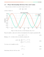
The angle or phase of a complex number is its angular distance from 0 degrees, which is 3 o’clock on a clock face. The angle also describes the relationship between the sine and cosine component of a complex exponential if the complex number was treated as the hypotenuse of a triangle.
Mathematically the arctangent is used to calculate the angle of a complex number  where
where
(13) 
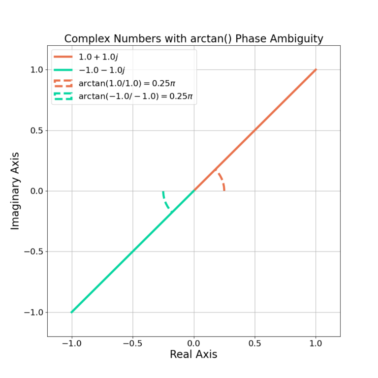
The  has a phase ambiguity due the division of
  . For example, the same angle is calculated when
  and
and  ,
,
(14) 
(15) 
although visually it can be seen in Figure 3 that the angles are not the same.
The phase ambiguity is resolved in software by treating the real and imaginary components as separate inputs as in MATLAB’s atan2() function or NumPy’s arctan2(). For example, using arctan2() is given in the following code snippet:
import numpy as np
c = 1 + 1j
print( np.arctan2( np.imag(c), np.real(c) ) )
c = -1 - 1j
print( np.arctan2( np.imag(c), np.real(c) ) )
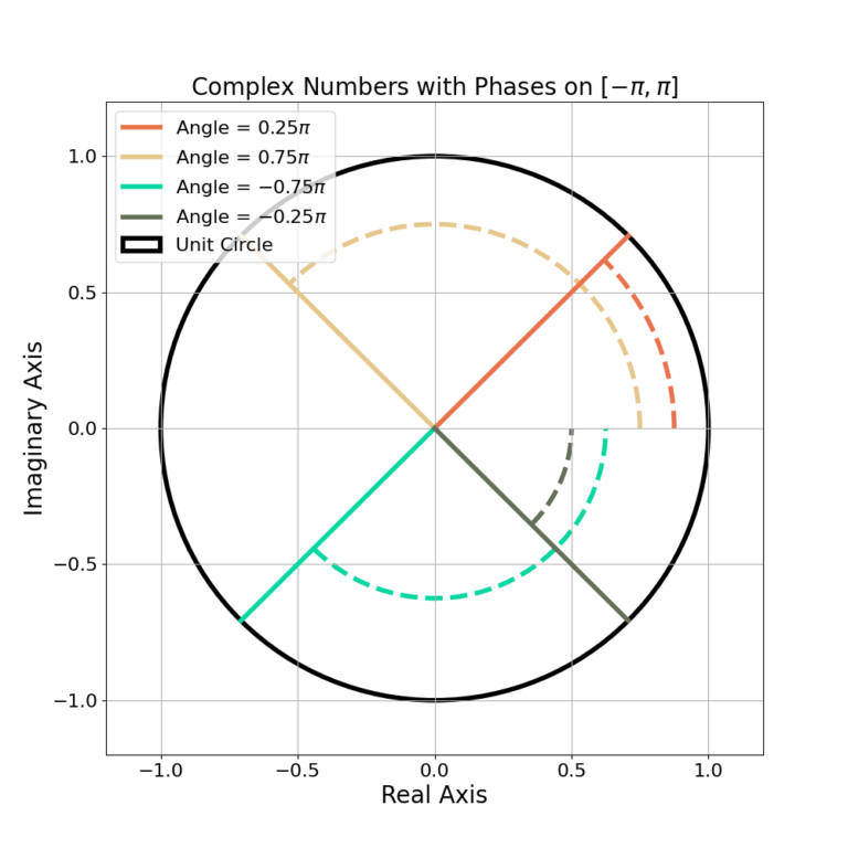
By convention the angle is measured from 0 degrees, and therefore
(16) 
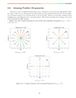
An example of angles plotted on ![[-\pi, \pi]](https://www.wavewalkerdsp.com/wp-content/ql-cache/quicklatex.com-92a990c704d7a8c7514a323d99652e8f_l3.png "Rendered by QuickLaTeX.com") is given in Figure 4.
is given in Figure 4.
The angle is periodic in  ,
,
(17) 
and may also be represented by
(18) 
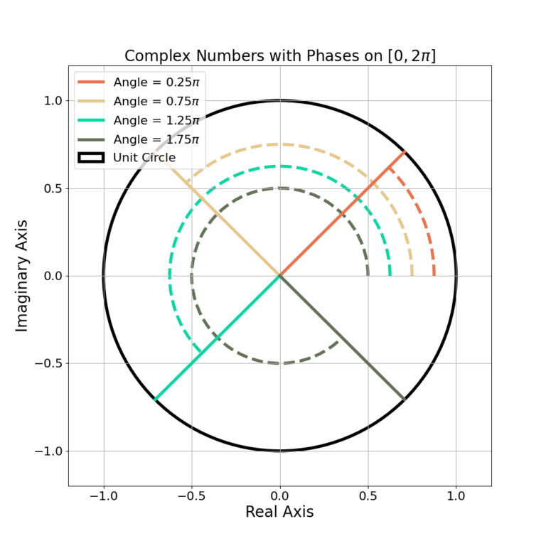
An example of angles plotted on ![[0, 2\pi]](https://www.wavewalkerdsp.com/wp-content/ql-cache/quicklatex.com-dbb0f8663da9b7c9b605f90189c76eea_l3.png "Rendered by QuickLaTeX.com") is given in Figure 5.
is given in Figure 5.
Polar form is most commonly used mathematically (pen and paper) due to its simplified multiplication. Almost all useful DSP functions require complex multiplication and therefore the polar form is the most common when working through the mathematics manually.
The polar form of complex number c given by
(19) 
where A is the amplitude and  is the phase. The complex number can be represented in polar form by
(20) 
Conjugation  negates the imaginary element of a complex number such that
(21) 
For , the conjugate is given by
(22) 
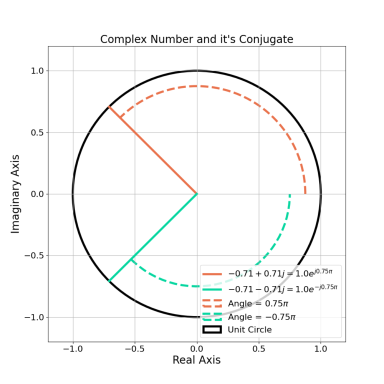
Conjugation is also the mirroring of c across the imaginary axis. Figure 6 gives an example of a complex number and it’s conjugate in the complex domain.
The conjugation operation does not effect the magnitude of a complex number ,
(23) 
Conjugation negates the angle of a complex number,
(24) 
The addition of complex numbers c and z,
(25) 
(26) 
is given by
(27) 
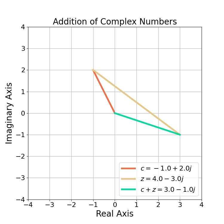
The addition of complex numbers is most easily done with Cartesian form rather than polar form. Adding complex numbers sums the real and imaginary portions separately (as they are orthogonal to one another) which can be visualized in Figure 7.
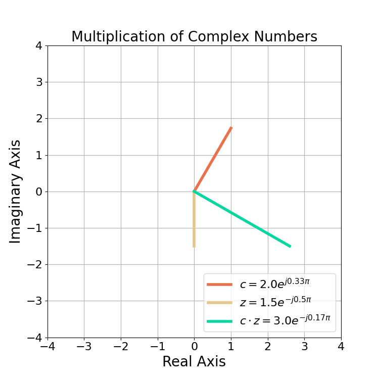
The multiplication of complex numbers c and z,
(28)
(29)
is given by
(30) 
The multiplication of (30) is clunky due to the distribution of the multiplication across multiple terms and can be simplified by converting both terms to polar first.
The multiplication of two complex numbers  and
and  is given by
(31) 
Figure 8 gives an example for  and
and  where
where