Wave Walker DSP

DSP Algorithms for RF Systems

Buy the Book!

DSP for Beginners: Simple Explanations for Complex Numbers! The second edition includes a new chapter on complex sinusoids.

Efficient Real to Complex Conversion with a Half Band Filter

December 15, 2021

Introduction

You are going to have to perform a real to complex conversion at some point in your DSP career. The most common way is having to convert samples from a real analog to digital converter (ADC) to complex baseband. There are different ways to implement real to complex conversion however this algorithm is particularly efficient by downconverting from $f_s/4$ using only a handful of multiplies. Additional computational savings will come from the decimate by 2 half band filter to remove the negative frequency spectral image.

Note: I have heard of this algorithm referred to as a “quad-band downconverter” but I have not been able to find it elsewhere. (I have looked in all the books I have, internet searches, etc.) If you have a reference for it or the correct name please leave a comment below or send me an email (matt@wavewalkerdsp.com).

Real to Complex Downconversion from fs/4

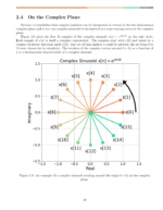
Complex downconversion is accomplished by multiplying a complex exponential c[n] against real samples $x_{R}[n]$

(1) $\begin{equation*}y[n] = x_{R}[n] \cdot c[n]\end{equation*}$

where

(2) $\begin{equation*}c[n] = e^{-j2\pi \frac{f}{f_s}n}.\end{equation*}$

The complex downconversion can be done from any frequency f but using $f=f_s/4$ is uniquely efficient which will be explained shortly. The frequency fs/4 is normalized by

(3) $\begin{equation*}\frac{f_s/4}{f_s} = 1/4\end{equation*}$

such that

(4) $\begin{equation*}c[n] = e^{-j2\pi \frac{f_s/4}{f_s} n}\end{equation*}$

which is simplified to

(5) $\begin{equation*}c[n] = e^{-j\pi n/2}.\end{equation*}$

Calculating (5) for multiple values of n produces a pattern

(6) $\begin{equation*}\begin{split}c[0] & = 1, \\c[1] & = -j, \\c[2] & = -1, \\c[3] & = j, \\c[4] & = 1, \\c[5] & = -j, \\c[6] & = -1, \\c[7] & = j.\end{split}\end{equation*}$

The pattern in the complex exponential (6) can therefore be simplified as

(7) $\begin{equation*}c[n] = \begin{cases}1 & n = 0, 4, 8, \dots \\-j & n = 1, 5, 9, \dots \\-1 & n = 2, 6, 10, \dots \\j & n = 3, 7, 11, \dots \\\end{cases}.\end{equation*}$

The downconversion output y[n] is therefore

(8) $\begin{equation*}y[n] = x_{R}[n] \cdot c[n] =\begin{cases}x_{R}[n] & n = 0, 4, 8, \dots \\-jx_{R}[n] & n = 1, 5, 9, \dots \\-x_{R}[n] & n = 2, 6, 10, \dots \\jx_{R}[n] & n = 3, 7, 11, \dots \\\end{cases}.\end{equation*}$

Multiplications of 1, -j, -1 and j in (8) can be implemented without multiplication which makes the processing much more efficient. The following block of Python code describes the multiplier-less downconversion:

# perform quad-band downconversion complexBasebandWithImage = np.zeros(len(receiveSignal),dtype=complex) for index in range(len(receiveSignal)): if (np.mod(index,4) == 0): complexBasebandWithImage[index] = receiveSignal[index] elif (np.mod(index,4) == 1): complexBasebandWithImage[index] = -1j*receiveSignal[index] elif (np.mod(index,4) == 2): complexBasebandWithImage[index] = -receiveSignal[index] else: complexBasebandWithImage[index] = 1j*receiveSignal[index]

Note: The multiplication by j may be necessary in software but would not be necessary in a hardware or FPGA implementation.

Real to Complex Example

Figure 1 is the time domain of a BPSK signal at real baseband and Figure 2 is the frequency response.

The real signal of Figure 1 is then upconverted to passband and noise is added which mimics a radio receiver with a real ADC, which will be referred to as the receive signal. Figure 3 is the time domain of the receive signal and Figure 4 is the frequency response.

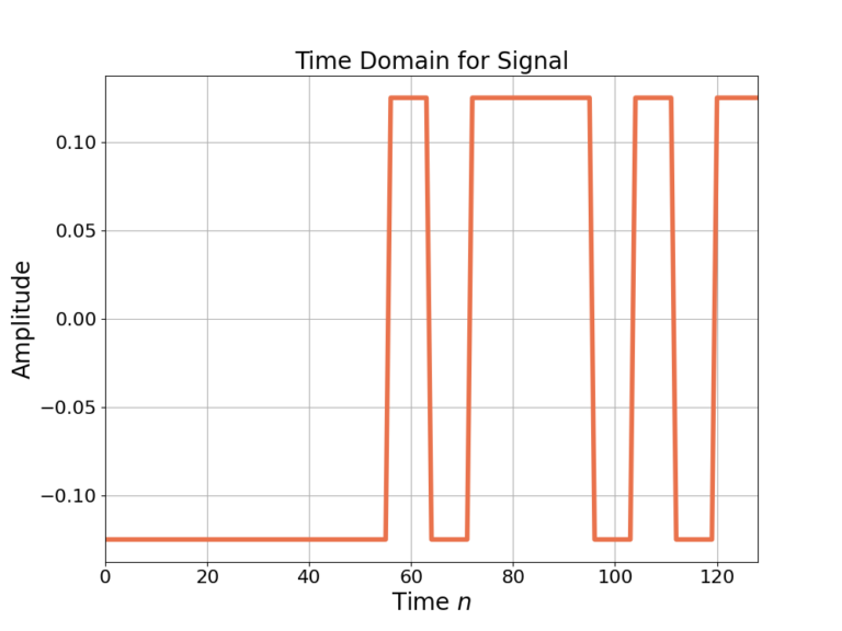
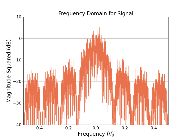
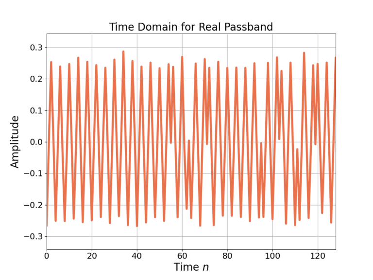
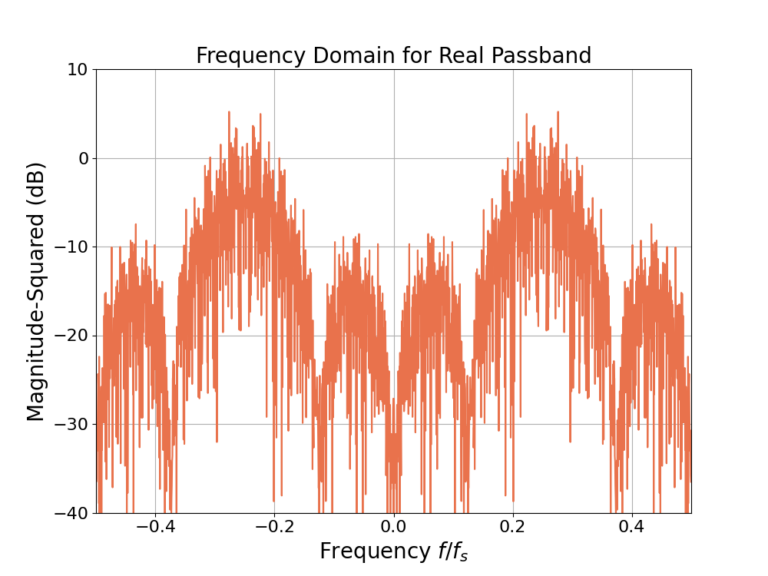
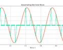
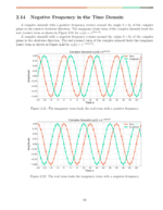
As the time domain signals in Figure 1 and Figure 3 are real, the magnitudes of their frequency responses in Figure 2 and Figure 4 are mirror images across f=0 [oppenheim1999, p.56].

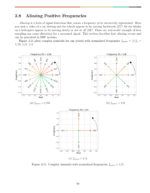
Figure 3 and Figure 4 is typically where an FPGA or hardware implementation of the quad-band downconverter would take place although it is simulated in Python for illustrative purposes. The downconversion to complex baseband shifts the signal centered at $f/f_s=1/4$ to $f/f_s = 0$ as in Figure 5 and Figure 6.

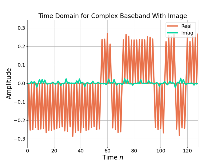
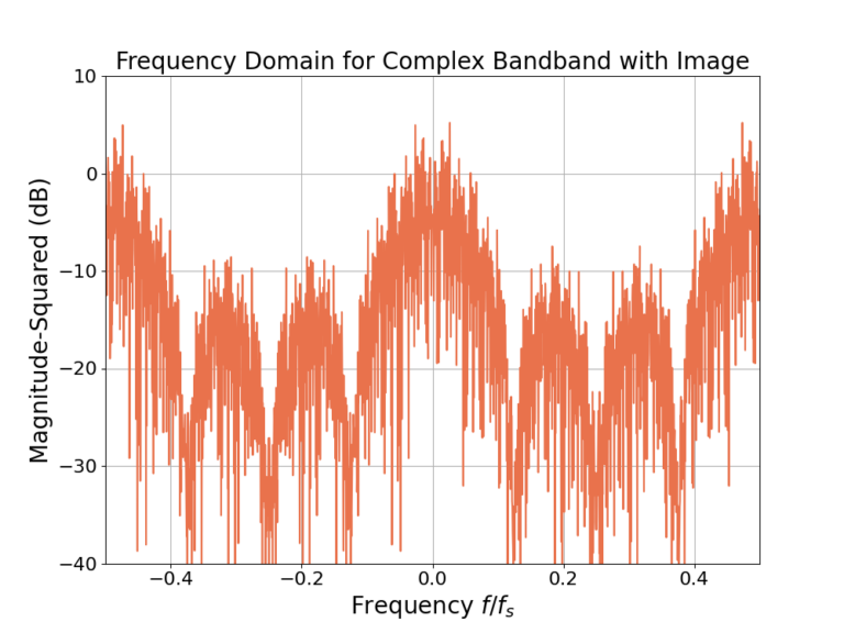
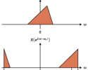
Comparing the signal in Figure 1 against the downconverted receive signal in Figure 5 shows two major differences: noise (which is to be expected in reception) and a high frequency component in each of the symbols. Figure 6 shows the high frequency component is a spectral copy shifted due to the downconversion. The downconverted signal is also now complex therefore the magnitude of the frequency responses is no longer symmetric across f=0 which can be seen in Figure 6 if you look closely.

Image Rejection Filter

Figure 6 shows two spectral copies of the same content: one image from -0.25 < f < 0.25 and another for -0.5 < f< -0.25 and 0.25 < f < 0.5. A low-pass filter is needed to reject the high frequency image. As the cut-off frequency should be $f/f_s = 0.25$ a half band filter will be used.

A previous post described how to design a half band filter and gave a downloadable script in Python for designing the filter weights. A half band filter is designed with a filter length of 19 weights an a transition bandwidth of 0.2. Figure 7 is the time domain and Figure 8 is the magnitude of the frequency response after filtering.

The half band filter has suppressed the high frequency contents of the complex baseband signal such that their impact is negligible. Nyquist’s theorem states that a signal’s information content is completely captured as long as the highest frequency in the signal is less than or equal to half the sampling rate. While the power of the frequency content at high frequency $|f| > 0.25$ is non-zero, it is small enough to be ignored and thus the signal can be downsampled by 1/2 and still satisfy Nyquist’s theorem in a practical sense.

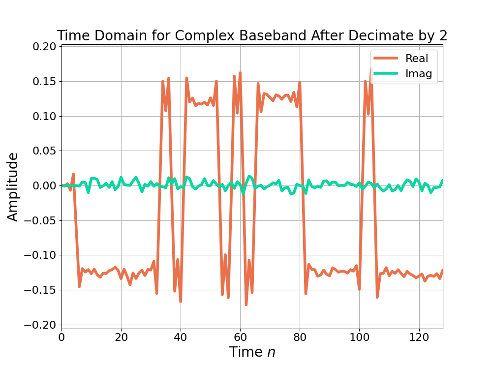
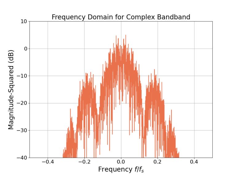
The time domain output of the half band filter after downsampling by 2 is shown in Figure 9 and the magnitude of the frequency response in Figure 10.

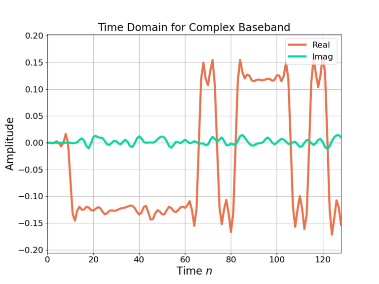
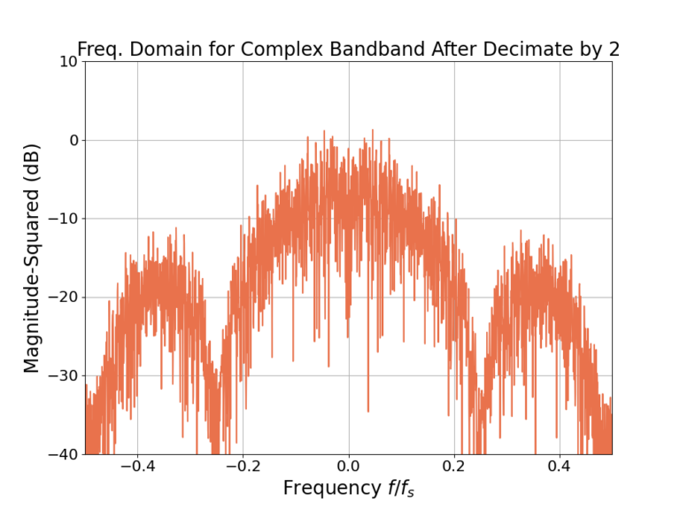
The decimation by 2 has contracted the time axis by a factor of 2 in Figure 9 when comparing against Figure 1 and Figure 5. Conversely the bandwidth of the signal has been expanded by a factor of 2.

The implementation of the decimate by 2 half band filter was implemented in a naive way for illustrative purposes but a highly efficient folded polyphase filterbank can be used instead. A folded polyphase filterbank implementation of the decimate by 2 half band filter can be implemented with $1/8^{th}$ of the multiplies as the naive approach. For example the filter in this example has 23 weights would require 23 complex multiplies for each input sample for the naive approach. The efficient folded polyphase filterbank would be reduced to $23/8 = 2.875$ complex multiplies per input sample!

Conclusion

Efficient real to complex conversion is an important part of building a receiver. Often radio receivers will have a single real ADC which will provide real samples which need to be converted into complex baseband where DSP algorithms typically operate. Real to complex conversion can be done in an efficient manner by downconverting from $f_s/4$ and using a folded polyphase filterbank to decimate by 2.

Have you seen the other posts on the half band filter?

Got a DSP question? DM me on Twitter @WaveWalkerDSP and I may make a blog post on it!

Wave Walker DSP

DSP Algorithms for RF Systems

Trending

Buy the Book!

Table of Contents

Introduction

Real to Complex Downconversion from fs/4

Real to Complex Example

Image Rejection Filter

Conclusion

Related

Leave a ReplyCancel reply