Wave Walker DSP

DSP Algorithms for RF Systems

Most Popular

Buy the Book!

DSP for Beginners: Simple Explanations for Complex Numbers! The second edition includes a new chapter on complex sinusoids.

Comb Filter Introduction and Analysis
March 1, 2023

Table of Contents

Introduction

A comb filter is a multiplier-less filter, meaning it only uses additions when computing the impulse response. The comb filter is one of the two major building blocks in the cascaded integrator comb (CIC) filter.

This blog post will describe both the impulse response and frequency response of the comb filter and demonstrate how to analyze the comb filter in the frequency domain.

Related DSP blogs:

Comb Filter Time Domain

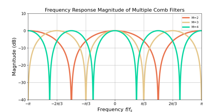
The difference equation for the comb filter is defined by [harris2021,p.395]:

(1)   \begin{equation*}y[n] = x[n] + x[n-M]\end{equation*}

where M > 0 which is the delay between the two samples being added.

Comb Filter Frequency Domain

It is difficult to assertain the impact of the filter only looking at the time domain in (1) but transformation into the frequency domain can make the analysis easier. Apply the Z-transform:

(2)   \begin{equation*}Y(z) = X(z) + X(z) z^{-M}\end{equation*}

and combine like terms:

(3)   \begin{equation*}Y(z) = X(z)\left( 1 + z^{-M}\right).\end{equation*}

The transfer function H(z) is therefore

(4)   \begin{equation*}H(z) = 1 + z^{-M}.\end{equation*}

Substituting z = e^{j\omega}, the frequency response is therefore

(5)   \begin{equation*}H\left( e^{j\omega} \right) = 1 + e^{-j\omega}.\end{equation*}

The magnitude-squared of the the frequency response is therefore

(6)   \begin{equation*}\begin{split}\left| H\left( e^{j\omega} \right) \right|^2 & = \left(1 + e^{-j\omega M}\right)\cdot \left(1 + e^{-j\omega M}\right)^* \\& = (1 + e^{-j\omega M}) \cdot (1 + e^{j\omega M}) \\& = 1 + e^{-j\omega} + e^{j\omega} + 1 \\& = 2 + e^{j\omega M} + e^{-j\omega M}.\end{split}\end{equation*}

Using Euler’s formula (6) can be written as 

(7)   \begin{equation*}\begin{split}\left| H\left( e^{j\omega} \right) \right|^2 &  = 2 + \frac{2}{2}\left( e^{j\omega M} + e^{-j\omega M}\right) \\& = 2 + 2 \cos\left( \omega M \right).\end{split}\end{equation*}

Comb Filter Passband Analysis

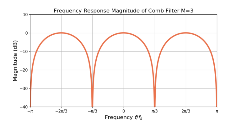
The maximum values, or pass-bands, of the comb filter’s frequency response (7) occur when 

(8)   \begin{equation*}\cos \left(\omega M\right) = 1\end{equation*}

such that

(9)   \begin{equation*}\left| H\left( e^{j\omega} \right) \right|^2 = 4.\end{equation*}

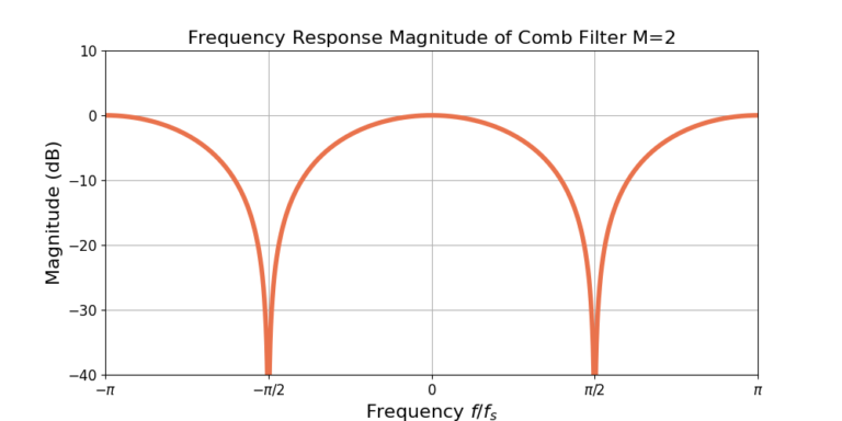
Using an example to illustrate (8), a comb filter with a delay M=2 will have maxima when

(10)   \begin{equation*}\cos\left( 2 \omega \right) = 1.\end{equation*}

Substituting \phi = 2\omega,

(11)   \begin{equation*}\cos \left( \phi \right) = 1\end{equation*}

when

(12)   \begin{equation*}\phi = 0, \pm 2\pi,\end{equation*}

therefore the maxima of the passband occur at

(13)   \begin{equation*}\omega = 0, \pm \pi.\end{equation*}

The values of \omega in (13) are limited to

(14)   \begin{equation*}-\pi \le \omega \le \pi\end{equation*}

because it is a discrete-time filter and -\pi and \pi correspond to the negative sampling frequency and positive sampling frequency in radians.

Comb Filter Stopband Analysis

The minimum values, or stop-bands, of the comb filter’s frequency response occur when

(15)   \begin{equation*}\cos \left(\omega \right) = -1\end{equation*}

such that

(16)   \begin{equation*}\left| H\left( e^{j\omega} \right) \right|^2 = 0.\end{equation*}

Using an example to illustrate (15), a comb filter with a delay M=2 will have minima when

(17)   \begin{equation*}\cos\left( 2 \omega \right) = -1.\end{equation*}

Substituting \phi = 2\omega,

(18)   \begin{equation*}\cos \left( \phi \right) = -1\end{equation*}

when

(19)   \begin{equation*}\phi = \pm \pi,\end{equation*}

therefore the minima of the passband occur at

(20)   \begin{equation*}\omega = \pm \frac{\pi}{2}.\end{equation*}

Examples of Comb Filter Frequency Responses

The magnitude of the frequency response of a comb filter with M=2 is given in Figure 1. Compare the result in Figure 1 against the result of the passband and stopband analysis in (13) and (20).

Figure 1: The magnitude of the frequency response of a comb filter for M=2. Note that the response has been normalized for 0 dB gain at omega=0.

Increasing the delay M results in more passbands and more stopbands. Figure 2 gives the magnitude of the frequency response for M=4.

Figure 2: The magnitude of the frequency response of a comb filter for M=3. Note that the response has been normalized for 0 dB gain at omega=0.

Figure 3 gives the responses for three different comb filters: M=2, 3 and 4. Increasing the delay M results in more maxima and more minima, which appear as more teeth in the comb. Increasing the delay M also narrows the teeth of the comb.

Figure 3: Increasing the delay M increases the number of teeth in the comb filter and reduces their width. Note that the magnitude has been normalized to 0 dB gain at omega=0.

Conclusion

The comb filter is multiplier-less filter, making it efficient to implement. The comb filter is also one half of the cascaded integrator comb (CIC) filter. The blog described both the impulse response and frequency response of the comb filter. Analysis was also performed on the passbands and stopbands of the frequency response.

Related DSP blogs:


God, the Lord, is my strength; he makes my feet like the deer’s; he makes me tread on my high places. Habakkuk 3:19

One Response

Leave a Reply

This website participates in the Amazon Associates program. As an Amazon Associate I earn from qualifying purchases.