Wave Walker DSP

DSP Algorithms for RF Systems

Buy the Book!

DSP for Beginners: Simple Explanations for Complex Numbers! The second edition includes a new chapter on complex sinusoids.

Is the Nyquist Sampling Rate Satisfied? (Homework Problem)

March 2, 2022

Introduction

In this blog I answer a question I received about how to apply Nyquist’s sampling rate mathematically and thought it’s worth sharing. One of the difficult parts about getting started in DSP is the concepts are not intuitive which is further compounded by the requirement that the early work must done mathematically, rather than by building or simulating. Take heart if you feel this way, you are not alone! I hope this blog is useful in helping to understand the mathematics of DSP. Please leave a comment below with other questions you have.

More blogs on sampling and DSP math:

Homework Question

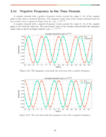
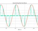
A continuous-time signal $x_{0}(t) = \sin\left( 2\pi f_{0} t)$ is modulated by a second continuous-time signal $x_{1}(t) = \sin\left( 2\pi f_{1} t\right)$ such that

(1) $\begin{equation*}y(t) = x_{0}(t) \cdot x_{1}(t).\end{equation*}$

The resulting signal y(t) is sampled with period $T_s$ .

Questions:

For $f_0 = 5000$ Hz, $f_1 = 1000$ Hz, and $T_s = 0.00025$ seconds,

Write y(t) as the sum of two sines or cosines
Sample the continuous-time signal y(t) to produce the discrete-time signal y[n]
What is the Nyquist sampling rate needed to sample y(t)?
What is the sampling frequency being applied to y(t)?
Is the signal y(t) sampled below or above the Nyquist sampling rate?

Question 1: Modulated Sinusoids

A trigonometric identity can be used on the modulated, or multiplied, sinusoids to represent them as the sum of two cosines:

(2) $\begin{equation*}\text{sin}\left( \alpha \right) \text{sin} \left( \beta \right) = \frac{1}{2} \left( \text{cos}\left( \alpha - \beta) - \text{cos}\left( \alpha + \beta \right) \right).\end{equation*}$

Substituting $\alpha = 2\pi f_{0} t$ and $\beta = 2\pi f_{1} t$ the signal y(t) can be written as

(3) $\begin{equation*}\begin{split}y(t) & = \frac{1}{2} \left( \text{cos} \left( 2\pi f_{0}t - 2\pi_f{1}t \right) - \text{cos} \left( 2\pi f_{0}t + 2\pi f_{1}t \right) \right) \\& = \frac{1}{2} \left( \text{cos} \left( 2\pi \left( f_{0} - f_{1} \right) t \right) - \text{cos} \left( 2\pi \left( f_{0} + f_{1} \right) t \right) \right)\end{split}\end{equation*}$

The multiplication of the two sines of frequency $f_{0}$ and $f_{1}$ resulted in the addition of two cosines, with frequency $f_{0} - f_{1}$ and $f_{0} + f_{1}$ .

Question 2. Sampling a Continuous-Time Signal

The continuous-time t is converted into discrete-time by $n T_s$ where $n = 0, 1, 2, 3, \dots~$ . The quantity $n T_s$ therefore represents the $n^{th}$ sampling instance at time $t = 0, T_s, 2T_s, 3T_s, \dots ~$ .

Discrete-time is represented by the time index n such that the discrete-time signal is y[n]. The continuous-time signal y(t) is sampled by indexing with $n T_s$

(4) $\begin{equation*}\begin{split}y[n] & = y\left( n T_s \right) \\& = \frac{1}{2} \left[ \text{cos} \left( 2\pi \left( f_{0} - f_{1} \right) t \right) - \text{cos} \left( 2\pi \left( f_{0} + f_{1} \right) t \right) \right] \\& = \frac{1}{2} \left[ \text{cos} \left( 2\pi \left( f_{0} - f_{1} \right) n T_s \right) - \text{cos} \left( 2\pi \left( f_{0} + f_{1} \right) n T_s \right] \right)\end{split}\end{equation*}$

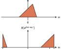
Question 3: Finding the Nyquist Sampling Rate

Nyquist’s theorem states that to avoid distortion the sampling frequency $f_{Nyq}$ must be greater than twice the largest frequency $f_{max}$ of the signal to be sampled, $f_{Nyq} > 2 f_{max}$ . The sampled signal (4) has two frequencies,

(5) $\begin{equation*}f_{0} - f_{1} = 5000 - 1000 = 4000~\text{Hz}\end{equation*}$

(6) $\begin{equation*}f_{0} + f_{1} = 5000 + 1000 = 6000~\text{Hz}.\end{equation*}$

The larger of the frequencies is $f_{max} = 6000$ and the minimum sampling frequency $f_{Nyq}$ needed to sample the signal without distortion is therefore

(7) $\begin{equation*}f_{Nyq} > 2 f_{max} = 2 \cdot 6000 = 12,000~\text{Hz}.\end{equation*}$

Question 4: Calculating Sampling Frequency

Any time period and frequency are inverses of one another,

(8) $\begin{equation*}T = \frac{1}{f}\end{equation*}$

and equivalently,

(9) $\begin{equation*}f = \frac{1}{T}.\end{equation*}$

The sampling period $T_s$ is related to the sampling frequency

(10) $\begin{equation*}f_s = \frac{1}{T_s}\end{equation*}$

therefore the sampling frequency is

(11) $\begin{equation*}f_s = \frac{1}{0.00025~\text{seconds}} = 4000~\text{Hz}.\end{equation*}$

Question 5: Is Nyquist's Sampling Theorem Satisfied?

The sampling rate $f_{Nyq} > 12,000$ Hz is the minimum sampling rate needed to sample y(t) without distortion. However, the signal has been sampled by frequency $f_s = 4000$ Hz. Since $f_s < f_{Nyq}$ , the signal is undersampled and Nyquist’s sampling theorem is not satisfied.