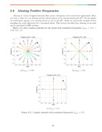
![Figure 6: The magnitude of the cross correlation between c[n] and y[n], |Ryc[tau]|.](https://www.wavewalkerdsp.com/wp-content/uploads/wordpress-popular-posts/5756-featured-125x100.png)
The output of a finite pulse response (FIR) filter h[n] is represented by convolution,
(1) ![\begin{equation*}y[n] = x[n] \circledast h[n],\end{equation*}](https://www.wavewalkerdsp.com/wp-content/ql-cache/quicklatex.com-433f869437bbad0153ee8a5d7a3f82bd_l3.png "Rendered by QuickLaTeX.com")
or alternatively,
(2) ![\begin{equation*}\begin{split}y[n] & = \sum_{k=-\infty}^{\infty} x[k] h[n-k] \\& = \sum_{k=-\infty}^{\infty} x[n-k] h[k].\end{split}\end{equation*}](https://www.wavewalkerdsp.com/wp-content/ql-cache/quicklatex.com-887250d4e5b71763f2f3d68a1e34c8f4_l3.png "Rendered by QuickLaTeX.com")
Figure 1 is an example of a FIR filter.
![Figure 1: The block diagram for an example FIR filter. Note that the filter weights h[n] have been time-reversed.](https://www.wavewalkerdsp.com/wp-content/uploads/2021/09/FIRFilterBlockDiagram-768x408.jpg)
From(2) it can be seen that x[k] is time reversed, x[-k], and delayed by n samples,
(3) ![\begin{equation*}x[n-k] = x[-k+n] = x[-(k-n)].\end{equation*}](https://www.wavewalkerdsp.com/wp-content/ql-cache/quicklatex.com-c4aba5e27d269b501275fa6342650356_l3.png "Rendered by QuickLaTeX.com")
Mathematically either x[n] or h[n] could be time reversed and delayed and the same output would be produced. However for easier analysis the convolution will be implemented by time reversing and delaying x[n].
Expanding (2),
(4) ![\begin{equation*}\begin{split}y[n] = \dots + h[-2]x[n+2] + h[-1]x[n+1] + h[0]x[n] + h[1]x[n-1] + \dots ~.\end{split}\end{equation*}](https://www.wavewalkerdsp.com/wp-content/ql-cache/quicklatex.com-504aa8bf32ce45685fd17337492b1edd_l3.png "Rendered by QuickLaTeX.com")
Delaying x[n] by T samples and substituting into (4) results in
(5) ![\begin{equation*}\begin{split}x[n-T] \circledast h[n] = \dots & + h[-2]h[n+2-T] + h[-1]x[n+1-T] + h[0]x[n-T] \\& + h[1]x[n-1-T] + h[2]x[n-2-T]\dots,\end{split}\end{equation*}](https://www.wavewalkerdsp.com/wp-content/ql-cache/quicklatex.com-2fb458e645f80c0319d06203a7f38f55_l3.png "Rendered by QuickLaTeX.com")
which can be simplified as
(6) ![\begin{equation*}y[n-T] = \sum_{k=-\infty}^{\infty} x[k-T] h[n-k],\end{equation*}](https://www.wavewalkerdsp.com/wp-content/ql-cache/quicklatex.com-301d5e675a028693a62d2c592e8af4dc_l3.png "Rendered by QuickLaTeX.com")
and
(7) ![\begin{equation*}y[n-T] = x[k-T] \circledast h[n].\end{equation*}](https://www.wavewalkerdsp.com/wp-content/ql-cache/quicklatex.com-6dc8a7210882bf345fec0cfcd5ba4ca0_l3.png "Rendered by QuickLaTeX.com")
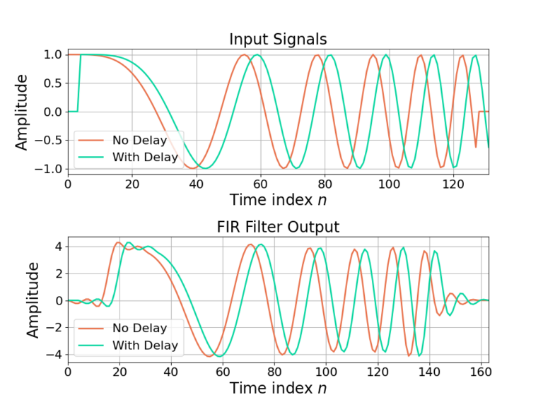
From (7) it can be seen that a delay in x[k] by T samples, x[k-T], results in a delay of the output y[n] by T samples, y[n-T] with no other affects. Figure 2 shows how a delay on an input signal results in the same delay in the output when filtered by a time-invariant FIR filter.
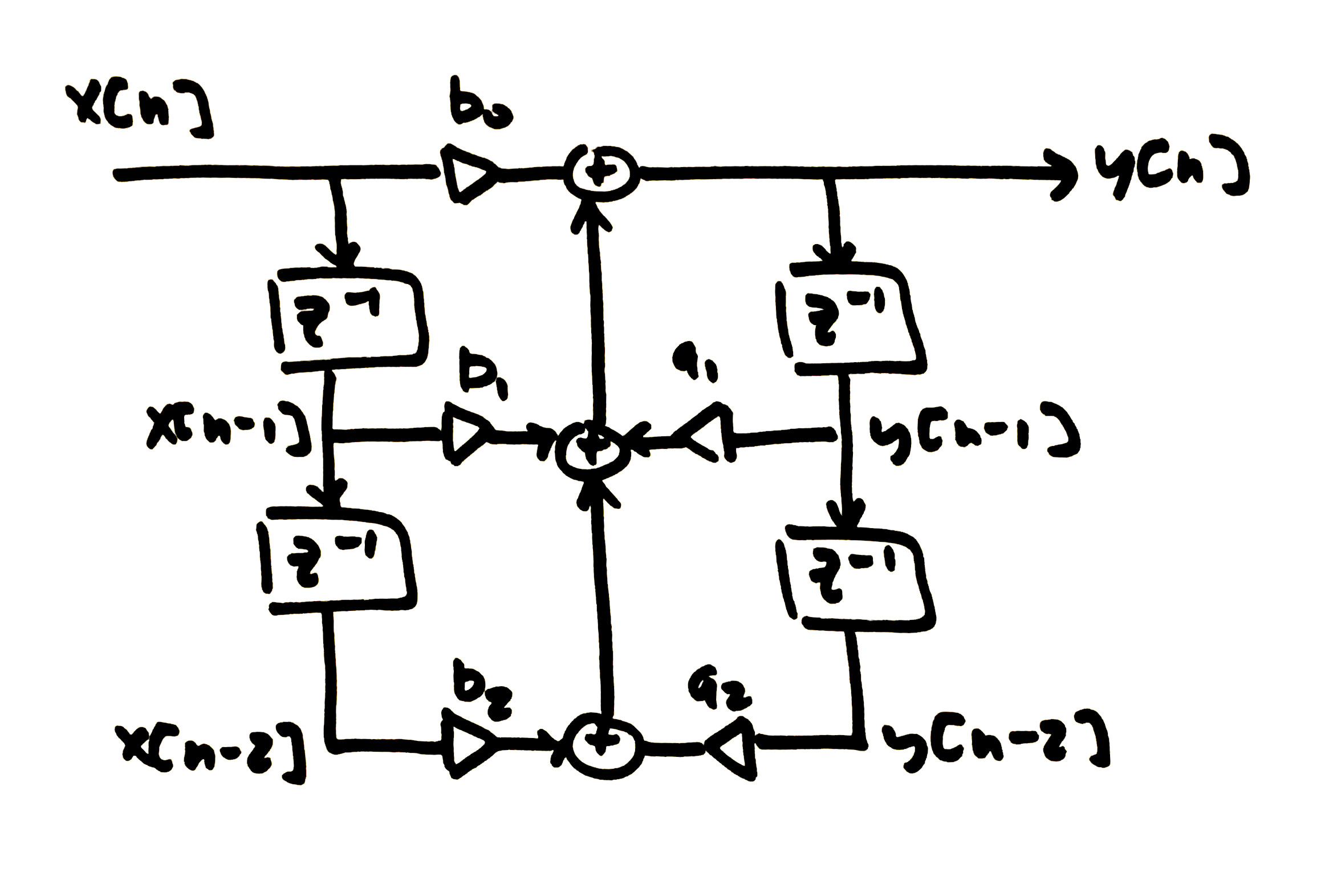
![\begin{equation*}y[n] = b_{0}x[n] + b_{1}x[n-1] + \dots + a_{1}y[n-1] + a_{2}y[n-2] + \dots\end{equation*}](https://www.wavewalkerdsp.com/wp-content/ql-cache/quicklatex.com-b281436cc8dcb268859f74dd2fb59b6f_l3.png "Rendered by QuickLaTeX.com")
![\begin{equation*}y[n] = \sum_{k=0}^{K-1} \left( b_{k}x[n-k] + \sum_{p=1}^{P-1} {a_{p}y[n-p] \right)\end{equation*}](https://www.wavewalkerdsp.com/wp-content/ql-cache/quicklatex.com-5483eea37f58401f5f4e55f85c898e4c_l3.png "Rendered by QuickLaTeX.com")
Delaying x[n] by T samples, x[n-T], such that  and substituting into (9) results in
(10) ![\begin{equation*}y[n-T] = \sum_{k=0}^{K-1} \left( b_{k}x[n-k-T] + \sum_{p=1}^{P-1} {a_{p}y[n-p-T] \right).\end{equation*}](https://www.wavewalkerdsp.com/wp-content/ql-cache/quicklatex.com-22e4bf6f8fa70fe11a0849808f8ff3be_l3.png "Rendered by QuickLaTeX.com")
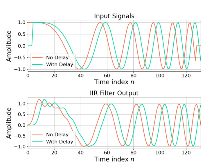
From (10), delaying x[n] by T results in the output being delayed by the same amount, y[n-T], with no other impact. The output y[n] is dependent on the input x[n] and the filter weights ak and bp. The filter weights ak and bp are constant for all time and therefore will not being time-varying. A delay of x[n] therefore corresponds directly to a delay in y[n]. Figure 4 gives an example of time-invariance in an IIR filter.
![Figure 5: Decimating by 2 consists of low-pass filtering with h[n] and then downsampling by 2.](https://www.wavewalkerdsp.com/wp-content/uploads/2021/09/decimateBy2BlockDiagram-scaled.jpg)
Combining the low-pass filtering with the downsampling operation will reveal the time-varying nature of the filtering operation and will produce computational efficiencies, referred to as a polyphase decimating filter. The low-pass filter output ![\bar{y}[n]](https://www.wavewalkerdsp.com/wp-content/ql-cache/quicklatex.com-1fa5f8204180bc64702a9d096f89ad2e_l3.png "Rendered by QuickLaTeX.com") can be written as
can be written as
(11) ![\begin{equation*}\begin{split}\bar{y}[n] & = x[n] \circledast h[n] \\& = \sum_{k} x[n-k]h[k].\end{split}\end{equation*}](https://www.wavewalkerdsp.com/wp-content/ql-cache/quicklatex.com-d289de60083f4d5d86bcdf74a4e27694_l3.png "Rendered by QuickLaTeX.com")
Downsampling by 2 discards every other sample. Mathematically, it allows for the opportunity to select even indices,
(12) ![\begin{equation*}y[n] = \bar{y}[2n]\end{equation*}](https://www.wavewalkerdsp.com/wp-content/ql-cache/quicklatex.com-c463138aa00e3429223e062b0476633c_l3.png "Rendered by QuickLaTeX.com")
or odd indices,
(13) ![\begin{equation*}y[n] = \bar{y}[2n+1].\end{equation*}](https://www.wavewalkerdsp.com/wp-content/ql-cache/quicklatex.com-18958a25088b51298b72026f6ffe9787_l3.png "Rendered by QuickLaTeX.com")
Both (12) and (13) are valid and only differ by delaying the input to the downsample by 1 sample. Choosing
(14) ![\begin{equation*}\bar{y}[2n]\end{equation*}](https://www.wavewalkerdsp.com/wp-content/ql-cache/quicklatex.com-dc488ed74a64384d3a3dec9214790d8d_l3.png "Rendered by QuickLaTeX.com")
and substituting (12) into (11) gives
(15) ![\begin{equation*}\bar{y}[2n] = \sum_{k} x[2n-k] h[k].\end{split}\end{equation*}](https://www.wavewalkerdsp.com/wp-content/ql-cache/quicklatex.com-8b4736f676983dd6a0cab4f05ca745f4_l3.png "Rendered by QuickLaTeX.com")
The filter h[n] produces a single output for each input x[n]. However, the downsampling by 2 operation discards all of the odd indices ![\bar{y}[2n+1]](https://www.wavewalkerdsp.com/wp-content/ql-cache/quicklatex.com-bbb2834b8ecf78237a917d22d255c0e3_l3.png "Rendered by QuickLaTeX.com") wasting the computation. The filter h[n] will be rearranged into a polyphase structure to avoid wasting the computation and making the decimation more efficient.
wasting the computation. The filter h[n] will be rearranged into a polyphase structure to avoid wasting the computation and making the decimation more efficient.
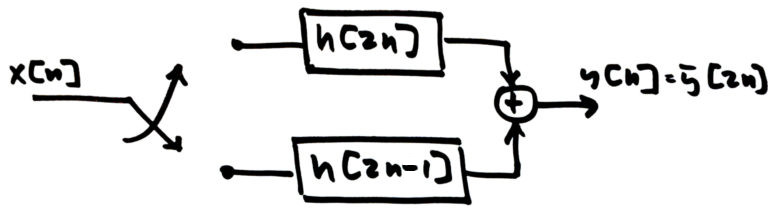
The filter output is arranged into even time indices x[2n] and odd time indices x[2n+1].
(16) ![\begin{equation*}\begin{split}\bar{y}[2n] & = \sum_{k ~ \text{even}} x[2n-k]h[k] + \sum_{k ~ \text{odd}} x[2n-k]h[k] \\& = \sum_{k} x[2(n-k)]h[2k] + \sum_{k} x[2(n-k)+1]h[2k-1] \\& = \sum_{k} x[2(n-k)]h[2k] + x[2(n-k)+1]h[2k-1] \\\end{split}\end{equation*}](https://www.wavewalkerdsp.com/wp-content/ql-cache/quicklatex.com-4c6a81e8e4952cda9ee3e5a0174bfffd_l3.png "Rendered by QuickLaTeX.com")
From (16) it can be seen that the even input samples x[2(n-k)] are filtered by the even filter weights h[2k] while the odd input samples x[2(n-k)+1] are filtered by the odd filter weights h[2k-1]. The time index of the input samples x[n] therefore indicates which set of filter weights will be applied. Figure 6 gives the polyphase partitioning and shows how the input switch for x[n] controls which filter weights will be applied.