Basic Rules for Complex Numbers
The mathematics of DSP and complex numbers can be confounding.
Understanding how  was difficult when I first started my DSP education and it’s still not something I fully grasp. When starting out in your DSP education sometimes it is enough to simply understanding how the tools and procedures are applied, rather than how they are derived.
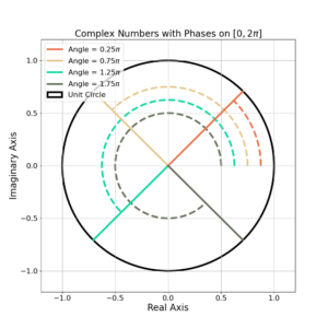
How Euler’s Formula Relates Triangles, the Unit Circle and Complex Sinusoids
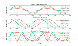
Sines and cosines are the foundation for representing signals and the affects of filters and therefore understanding their mathematics is one of the foundational tools for signal processing. Euler’s formula is a mathematically compact and useful representation used for representing complex sinusoids.
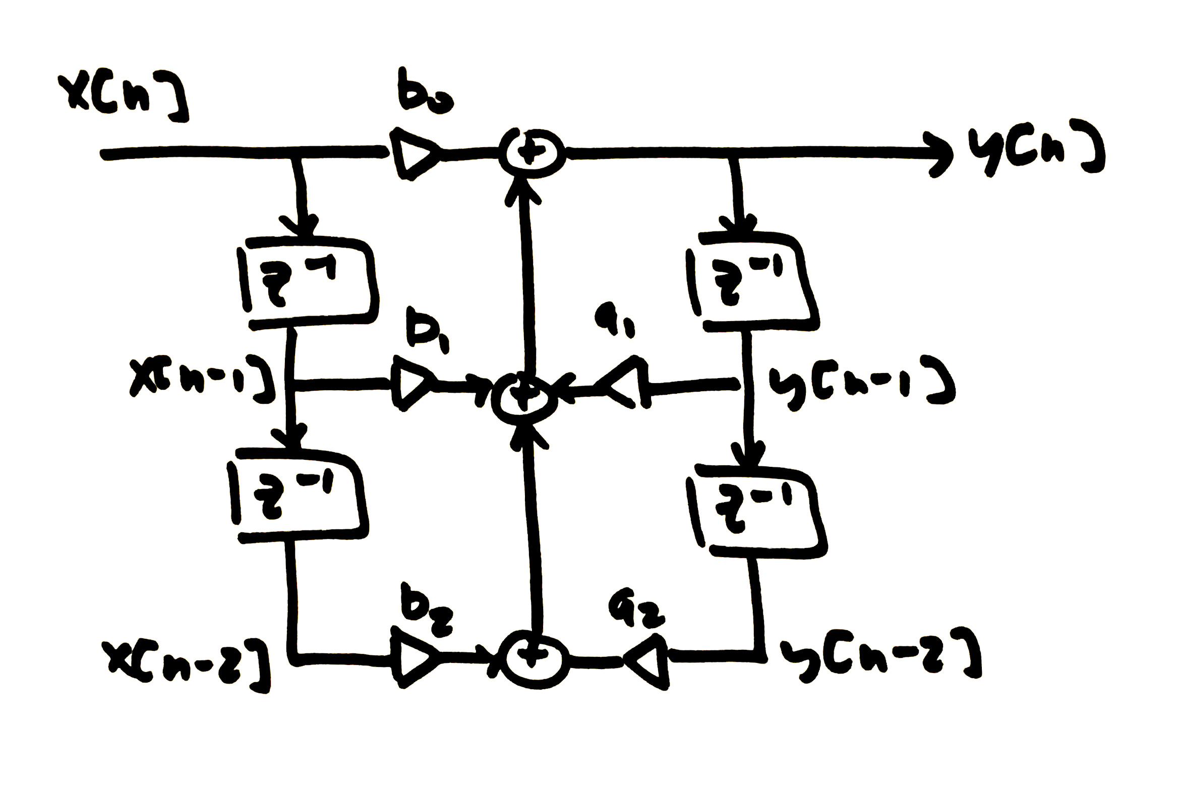
Time Invariant and Time Varying Filters
Introduction The response of time invariant filters is independent of time and have filter weights which do not change over time. Time invariance (TI) is
![Figure 1: A moving average filter is implemented by delaying the input signal x[n] and then scaling by 1/3 and summing all results.](https://www.wavewalkerdsp.com/wp-content/uploads/2021/09/movingAverageLength3-300x191.png)
Digital Signal Processing through the Lens of the FIR Filter
Digital signal processing has two components: signals and filters.
A signal is a time-series which has information (RF vocabulary) and filters are useful in applying a desired affect to a signal. These affects can be:
- enhancing information elements of a signal,
- attenuating or minimizing noise,
- or some other modification.
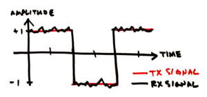
Signal and Noise: The Vocabulary of RF
All DSP scenarios will include a signal and noise.
But what are they? Using a common set of clearly defined terms is important to properly understand what information is trying to be conveyed.

WP QuickLaTeX for Running LaTeX on WordPress
Installing and operating WP QuickLaTex was quite puzzling for me, I hope the following instructions are useful!
Richard Hamming, Acorns and the Engineering Mindset
Richard Hamming was a pioneer in the fields of electrical engineering, computer engineering and computer science. You might not know he has also had a positive and significant impact on engineering culture with his talk “You and Your Research”.
Central Limit Theorem: Fact or Fiction?
Where were you when you first heard about the Central Limit Theorem (CLT)?
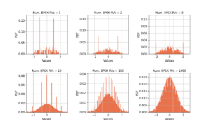
If you are like me, you heard of the CLT in the classroom as a justification for the assumption of Gaussian noise in the RF environment. The CLT states that the summation of independent random variables (RV) approaches a Gaussian distribution with an increasing number of random variables.
The CLT is convenient in simplifying mathematics, but when and how should it be used? Under what circumstances is it valid?
Let’s take a brief look at how well three different random variables follow the CLT.
Welcome to Wave Walker DSP!
Thanks for coming to Wave Walker DSP! I plan to bridge the gap between academic knowledge found in the classroom with the intuition of the