Wave Walker DSP

DSP Algorithms for RF Systems

New Book!

The third edition of DSP for Beginners: Simple Explanations for Complex Numbers! Includes a new chapter on sampling.

Phase relationship between sine and cosine

Barker Code Auto-Correlation Properties

March 1, 2024

Introduction

Barker codes are a special type of sequence which have excellent auto-correlation properties. This blog describes Barker codes, gives a mathematically example of the auto-correlation, and lists all of the auto-correlation magnitudes in figures.

Check out these blogs:

Barker Codes

A Barker Code is a sequence of length M whose maximum auto-correlation magnitude at time-lag $\tau = 0$ is M, and otherwise the auto-correlation magnitude is less than or equal to 1, such that

(1) $\begin{equation*}|R_{x}[\tau]| = M,\end{equation*}$

for $\tau = 0$ and

(2) $\begin{equation*}|R_{x}[\tau]| \leq 1,\end{equation*}$

for $\tau \neq 0$ .

There are a limited set of Barker codes:

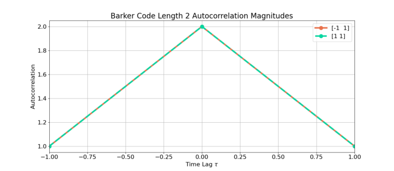
Length 2: [1, -1], [1, 1]
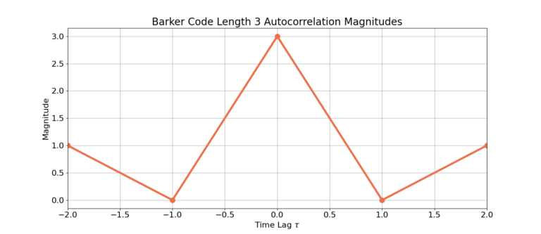
Length 3: [1, 1, -1]
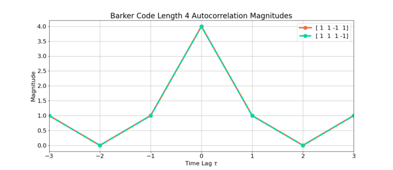
Length 4: [1, 1, -1, 1], [1, 1, 1, -1]
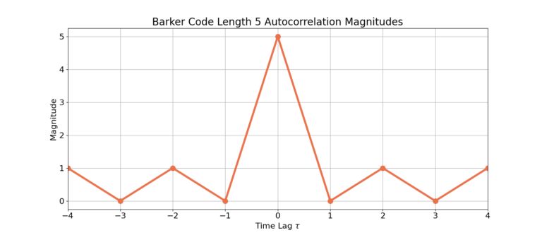
Length 5: [1, 1, 1, -1, 1]
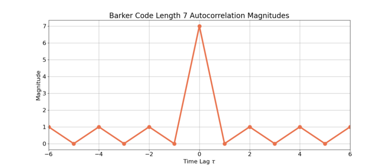
Length 7: [1, 1, 1, -1, -1, 1, -1]
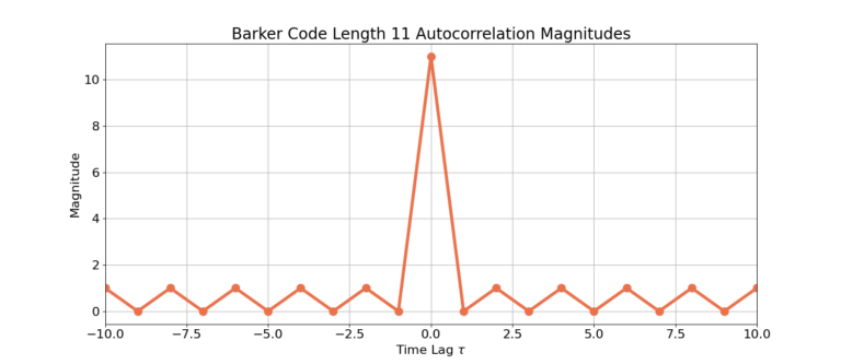
Length 11: [1, 1, 1, -1, -1, -1, -1, 1, -1, -1, 1, -1]
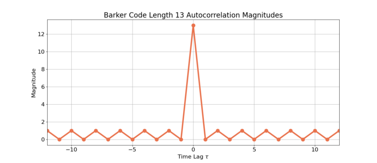
Length 13: [1, 1, 1, 1, 1, -1, -1, 1, 1, -1, 1, -1, 1]

Autocorrelation Mathematically

To demonstrate the auto-correlation properties of a barker code, let us work out an example using the length M=3 code which is 1, 1, -1. For background on autocorrelation, please review the blog: Cross Correlation Explained With Real Signals.

For time delay $\tau = 0$ the two signals will overlap perfectly and the auto-correlation is therefore computed by the element-by-element multiply, summing the result and taking the magnitude:

(3) $\begin{equation*}|R_{x}[0]| = |(1 \cdot 1) + (1 \cdot 1) + (-1 \cdot -1)| = 3,\end{equation*}$

which is equal to the length M=3.

For time delay $\tau = -1$ , one signal is delayed by 1 sample and the two sequences are multiplied and summed such that

(4) $\begin{equation*}|R_{x}[-1]| = |(1 \cdot 0) + (1 \cdot 1) + (-1 \cdot 1)| = 0.\end{equation*}$

For time delay $\tau = -2$ ,

(5) $\begin{equation*}\begin{split}|R_{x}[-2]| & = |(1 \cdot 0) + (1 \cdot 0) + (-1 \cdot 1)| \\ & = |-1| \\& = 1.\end{split}\end{equation*}$

For time delay $\tau = 1$ ,

(6) $\begin{equation*}|R_{x}[1]| = |(1 \cdot 1) + (1 \cdot -1) + (-1 \cdot 0)| = 0.\end{equation*}$

For time delay $\tau = 2$ ,

(7) $\begin{equation*}\begin{split}|R_{x}[2]| & = |(1 \cdot -1) + (1 \cdot 0) + (-1 \cdot 0)| \\& = |-1| \\& = 1.\end{split}\end{equation*}$

The auto-correlation magnitude $|R_{x}[\tau]|$ is therefore the sequence 1, 0, 3, 0, 1, which can be seen graphically in the following section.

Autocorrelation Plots

The following figures display the auto-correlation magnitudes for all of the Barker codes.

Conclusion

This blog lists the Barker codes, describes and demonstrates their auto-correlation properties mathematically, and displays the auto-correlation magnitudes for all sequences graphically.